Dense Linear Algebra

Problem

Some problems can be expressed in terms of linear algebraic operations over dense arrays of data vectors and matrices containing mostly non-zero values). How does one balance data movement and computation in order to maximize performance?

Context

Many problems are expressed in terms of linear operations on vectors and matrices. Common examples include solving systems of linear equations, matrix factorization, eigenvalue problems, and matrix multiplication. The way in which a real-world problem is expressed in terms of these basic linear algebra tasks can be influenced by:

1. the structure of the problem
2. how a continuous problem is sampled
3. how a general solution is expanded in terms of simpler basis functions

The pivotal problem in computational linear algebra is how to balance data access costs with the cost of computation. Given the disparity between memory and CPU speeds, it is critical to maximize the amount of computation carried out for each item of data accessed from memory. For problems for which the systems of equations associated with a problem are dense (i.e. they contain mostly non-zero values), it is often possible to exploit a surface to volume effect providing plenty of computation to hide the costs of accessing data. How do we write software that can take advantage of this property in order to achieve high performance?

Forces

Universal forces

• A solution to this problem needs to trade off the cost of recomputing intermediate results with storing them and fetching them later.

• Overlapping computation with data movement requires software constructed around the details of a particular memory hierarchy. But this is in direct conflict with the need to write portable software.

Implementation dependent

• A linear algebra operation may dictate a distinct layout of data to achieve optimal perfor- mance. These data layouts, however, may conflict with those needed by other operations forcing the programmer to balance data copy overheads with potentially sub-optimal algorithms.

Solution

Linear Algebra Libraries

Dense linear algebra problems benefit from the fact that they map onto a relatively modest collection of standard mathematical operations such as the symmetric eigenvalue problem, multiplication, or LU factorization. Hence, for many operations in linear algebra, a linear algebra library such as LAPACK[1] or ScaLAPACK[2] for distributed memory systems may provide all that is needed. If this is the case, the task faced by the programmer is how to define his or her data so the related matrices are in the format required by the math library.

BLAS Routines and Templates

If a linear algebra library exists for your platform, it can save you a lot of effort; however, if such a library does not exist or you have specialized needs, using preexisting linear algebra subroutines to perform basic operations such as matrix-matrix multiplication can save time and yield good performance. Many of the more advanced dense linear algebra tasks are built from the simple routines contained in a standard BLAS (Basic Linear Algebra Subroutines) library. The Templates series of books [3][4], which are freely available electronically, contain extensive information which guides the reader through the construction and organization of various linear algebra solvers from the BLAS.

BLAS libraries are available for most architectures on the market and encapsulate hardware specific assembly code often required to achieve high performance. There are three levels of BLAS:

• BLAS Level 1: Vector/Vector operations, O(N ) for data movement and computation
• BLAS Level 2: Vector/Matrix operations, O(N 2) for data movement and computation.
• BLAS Level 3: Matrix/Matrix operations, O(N 2) for data movement, O(N 3) for computation. The BLAS level 3 routines stand out because of the smaller order of complexity for data move-

ment (O(N 2)) than for computation (O(N 3)). Due to this fact, BLAS Level 3 routines can approach peak performance on most parallel systems. For this reason, a programmer would greatly benefit from structuring an algorithm to favor BLAS Level 3 functions. For example, replacing a large number of dot products (a BLAS level 1 function) with a single matrix-matrix multiplication (a BLAS level 3 function) can turn a problem bound by memory bandwidth into a compute-bound problem.

Auto-Tuned Libraries

If a BLAS library does not exist for the target architecture, there may still be hope. ATLAS (Automatically Tuned Linear Algebra Software) [5] and PHiPAC (Portable High Performance ANSI C)  [6] are two related projects which aim to automatically build and optimize BLAS routines for any architecture. Both rely on the concept of auto-tuning in order to achieve high performance without requiring any hand tuning or assembly coding. The auto-tuning process basically iterates through a large space of computational parameters and produces a library using the parameters which yielded the best performance on the target system.

Starting From Scratch

If none of the above suggestions are feasible, the task is too specialized, or for some reason you really want to start from scratch, it is important to understand how to structure computation in order to optimize utilization of the memory hierarchy. Because matrix multiplication is such an important building for many linear algebra routines, we will give an overview of its optimization here.

Naïve Approach

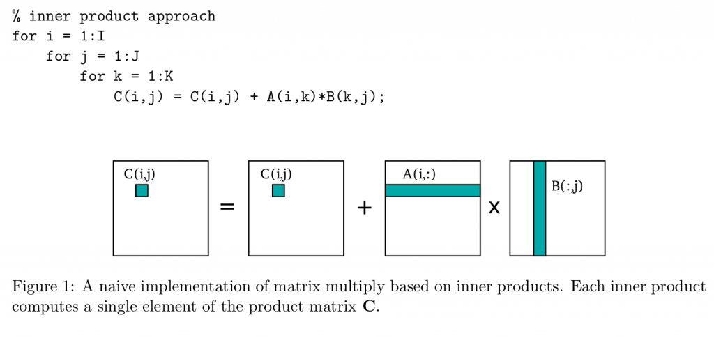
There are many ways to organize the computation of a basic matrix-matrix multiplication, written as:

C = C + AB

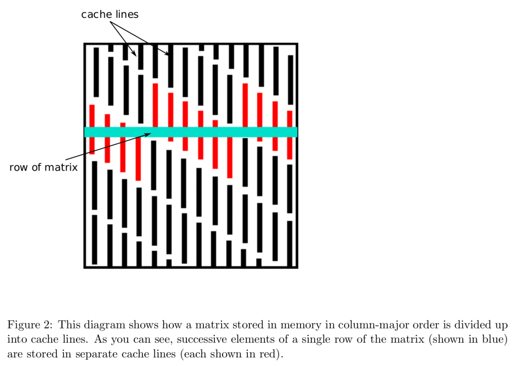
Na¨ıve implementations carry out an inner product for each element of the product matrix. This is shown as 3 nested loops in Figure 1. The problem with this na¨ıve approach is that it is highly suboptimal in terms of spatial locality. This is demonstrated in Figure 2 which shows how a matrix stored in column-major order will have adjacent row elements stored in separate cache lines. Accessing data in such a pattern can significantly increase data movement overhead.

Outer Product Approach

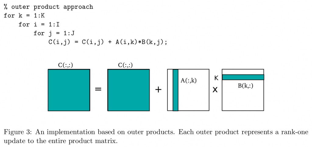
A better approach is based on outer products (shown in Figure 3), in which the product of a column of A and a row of B acts as a rank one update to the entire product matrix C.  Notice that even

though the k loop has been moved to the outer most level, the three nested loops still produce the same result. While this approach doesn’t solve the spatial locality problem, it can be utilized effectively in a blocked-based algorithm.

Blocked Approach

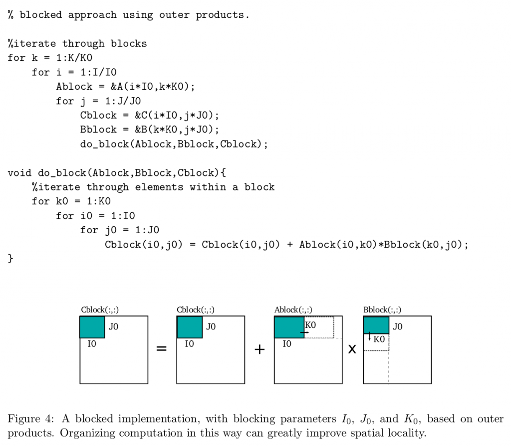
More sophisticated algorithms construct the product hierarchically from multiplications of smaller matrix blocks [7]. By computing outer products on small blocks of the input and output matrices, we can more effectively exploit spatial locality and data reuse. Figure 4 illustrates a blocking scheme with parameters I0, J0, and K0.

Auto-Tuning the Blocked Approach

When using a blocked approach, the optimal block sizes will change across architectures. Variables that can affect the best blocking parameters include the number of floating point registers, cache sizes, TLB size, time to access various levels of the memory hierarchy, number of floating point units, etc.. The interaction between all of these factors is so complicated that being able to decide on optimal blocking parameters while simply considering these variables is near impossible.

An effective way to arrive at optimal values for the blocking parameters, I0, J0, and K0, is through the use of auto-tuning. As mentioned above, ATLAS[5] and PHiPAC[6] are two examples

of the successes of auto-tuning matrix multiply. In simple terms, to auto-tune a blocked matrix multiply, one would simply write a script to compile the blocked code with many different com- binations of blocking parameters, measure the performance of each version of the code, and then choose the version that performed best.

One thing to be aware of when using a blocked approach is that many times, the optimal block size does not evenly divide the dimensions of the entire matrix. This can be handled in two ways. In the first method, one can simply zero pad the matrices up to a size that is divisible by the block size.  Alternatively, functions that use smaller-sized blocks can be written to handle the “fringes”.

Multiple Level Blocking

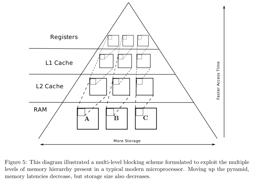
A first level of blocking, as discussed above, is commonly referred to as “register blocking” because the data reuse properties of such an approach are thought to exploit the speed of the processor registers. In order to more fully exploit additional levels of the memory hierarchy, multiple levels of blocking can be used. This concept is illustrated at a high level in Figure 5.

Code for using an additional level of blocking would iterate through all of the larger, second- level blocks contained in each matrix. Within the code to handle each second-level block, the code to iterate through the first-level blocks contained within the current second-level block would be called.

Using a second level of blocking is thought to exploit the L1 cache which is slower than the register but is much larger in size. Utilizing a third level of blocking would target the L2 cache. Subsequent levels of blocking, while possibly effective, are not typically used.

Additional Optimizations

1. Explicit Loop Unrolling

While some loop unrolling can automatically be done by the compiler, explicitly coding loops as unrolled can allow the compiler to use additional optimizations, ignore false dependencies,

2.   Use local variables to explicitly remove false dependencies

If matrix values are read into locally declared variables and these local variables are used in the calculations, the compiler will allow the program to proceed without incorrectly assuming that it needs to wait for the result of a previous update to a matrix element. Example in [6]

3.   Use SIMD instructions

Many architectures have vector instructions that can perform a single operation on multi- ple variable in a shorter amount of time than it would take to perform the operation on each variable individually. Matrix multiplication can greatly benefit from the use of such instructions.

Many more low level optimizations concerning pointer use, addressing, and reducing overall operations are covered in the PHiPAC paper.

Invariant

• The discrete representation of the problem (that leads to the matrices and vectors) accurately represents the original problem and produces well conditioned matrices.

• The final result approximates the mathematical definition to within tolerated round-off error.

Example

Computational Electromagnetics often leads to dense systems of linear equations. For example, in the late 1980s programs were developed to generate the radar cross section as a function of aircraft design parameters to reduce the signature of the aircraft (i.e. to support the design of stealth aircraft).

These simulations of electromagnetic fields use one of two numerical approaches:

1. Method of moments or boundary element method (frequency domain). This method produces large dense matrices.

1. Finite differences (time domain); which leads to large sparse matrices (which are sometimes solved by decomposing the sparse system into smaller dense matrices).

The numerical procedures are:

1. discretize the surface into triangular facets using standard modeling tools.
2. represent the amplitude of electromagnetic currents on the surface as unknown variables.
3. define integral equations over the triangular elements and discretize them as a set of linear equations.

At this point the integral equation is represented as the classic linear algebra problem:

Ax = b

where

A is the (dense) impedance matrix,

x is the unknown vector of amplitudes, and

b is the excitation vector.

Now that the problem is defined in terms of a system of equations, it can be solved using one of the many preexisting solvers.

Known Uses

Dense linear algebra is heavily used throughout the computational sciences. In addition to the electro-magnetics problem we just described, problems from quantum mechanics (eigenvalue prob- lems), statistics, computational finance and countless other problems are based on dense matrix computations. Sparse linear algebra is probably more common, but note that many sparse problems decompose into solutions over smaller dense matrices.

Related Patterns

This pattern is closely related to a number of lower level patterns depending on the direction taken in constructing the detailed solution.  Often, the geometric decomposition pattern is used in constructing parallel dense linear algebra problems. For matrices represented as hierarchical data structures, the divide and conquer pattern is indicated. The data structures used with dense linear algebra problems especially on NUMA or distributed memory systems are addressed in the Distributed arrays pattern. And finally, depending on the details of how a problem is represented, a problem can result in sparse instead of dense matrices (and hence the Sparse Linear Algebra pattern).