Backtrack Branch and Bound

We have an extremely large space which we need to search to make a decision or to find an optimal solution. The space is so large that enumerating every point in the space is infeasible. How do we search the space efficiently?

Both decision and optimization problem are search problems.

A decision problem is a problem of which the output is true or false. For example, SAT is a popular decision problem. Given a product of clauses, we need to decide whether there exists an assignment for all variables in the clauses such that the output of the function is 1. A clause is a sum over several variables. (a+b), (c+d), and (e+f) are clauses. The function (a+b)(c+d)(e+f) is satisfiable by the assignment a=1, c=1, e=1.

An optimization problem is a problem of which we want to maximize or minimize an objective function according to some constraints. For example, integer programming is a well-known optimization problem. Let A be an n by n matrix, b be an n by 1 vector, c be an n by 1 vector. The standard integer programming can be formulated as: min c^T x s.t. Ax ≤ b, x ∈ Z^n

A brute force approach to search such a space would try all possible points in the space to find the optimal solution. For example, when solving the SAT Problem, we can enumerate all the possible assignments on the variables. This approach will definitely find an optimal solution. However, the complexity of this approach is exponential in the size of the inputs. If the size of the input is large, it is not possible to try all inputs.

What are the factors that impact the solution of the problem?

1. the variables in the problem should have an ordering to allow complete and efficient exploration of the search space
2. the problem should have a self-similar or recursive structure (i.e. a problem with (n-2) elements is a smaller instance of a size (n) problem)
3. it is possible to approximate bounds for the optimal solution

Universal forces:

• One must balance the cost of computing the bounds with the amount of search space it prunes

Implementation forces:

• When parallelizing the search, it is easy to find independent search problems to execute. However, the more independent search problems we invoke, the harder it is to synchronize them. Since enumeration is impossible, the only way we will get traction on this problem is to use information derived during the search process to simplify the problem. The more search problems we invoke, the more difficult it becomes to do this, which forces the solution process towards enumeration.
• Exposing sufficient concurrency in the application to keep all the processing elements fully occupied, but exposing larger amount of concurrency increases parallel overhead
• Running time vs storage trade off. If we want to solve the problem efficiently, we can store all the subproblems up to date, and deal with the one that is most likely to solve the problem. However, it is very expensive to store all the subproblems. We can also choose the newest generated subproblem to deal with. We do not need to store a lot of subproblems under such case, but we might need to go through larger branches to solve the problem.

Search problems lend themselves to parallel implementation, since there are many points to search. However, since enumeration is too expensive computationally, the searches have to be coordinated in some way.

The solution is to use branch-and bound. Instead of exploring all possible points in the search space, we can repetitively divide the original problem into smaller subproblems, evaluate specific characteristics of the subproblems so far, set up constraints according to the information at hand, and eliminate subproblems that do not satisfy the constraints. By such procedure, the size of the feasible solution space will be reduced gradually. Consequently, we only need to explore a small part of the possible input combinations to find the optimal solution.

The branch-and-bound pattern has four basic operations.

1. Branching
2. Evaluation
3. Bounding
4. Pruning

Branch-and-Bound Operations

1) Branching: If a subproblem p cannot be solved directly, we decompose it into smaller subproblems p1, p2, …, pn.

In integer linear programming, we can branch on the non-integer variables, adding a constraint in each subproblem which forces a non integer variable to be an integer. More specifically, if the current solution has x1 = 3.5 for x1 which must be integer in the optimal solution, p1 can have a constraint that x1 ≤ 3, and p2 can have a constraint that x1 ≥ 4. These constraints define different subproblems.

Sometimes we can use heuristics for identifying branching variables (variables that will be branched). For example, we can order variables according to a heuristic cost function, and then branch the variables by the order we found. Given a SAT problem (A’+B’)(B’+C’)(A+C’), we can calculate the number of other variables that will be forced to be 0 if the variable is assigned value 1 as the cost function f(x). f(A)=1, f(B)=2, f(C)=1. Therefore, the ordering of the variables is BAC. We will branch on variable B first, A second, C last.

2) Evaluation: The application of the objective function to a point in the search space

For example: In integer linear programming, we need to decide whether the current solution is feasible first. If so, we need to calculate the objective function for the current solution. In SAT problem, we will verify whether the current solution satisfies the objective function.

3) Bounding : Given a subproblem p, calculate bounds on p. This may be done recursively. The bounding operation is key to the success for the branch and bound approaches. The bounding operation must be relatively efficient to evaluate (usually at most polynomial complexity in the size of the subproblem), and it must provide a bound on the best solution contained in the subproblem. If the bounding operation finds the actual best solution in the subproblem, we have found a current feasible point, which can be used globally for pruning other subproblems.

In branch and bound problems, we can find a way to derive upper and lower bounds on the solutions contained in the space by solving a simplified version of the search problem. When we are searching for a minimal point, we may use a upper bound to prune the search. Take integer programming as an example. Suppose that we are solving a minimization integer programming problem. By removing the constraints that all variables are integers, we will relax the original integer programming problem into a linear programming problem. The minimum value of the linear programming provides a lower bound of the integer programming problem. Whenever we found a feasible solution, it forms an upper bound of the integer programming problem. The optimal solution should be smaller than or equal to the feasible solution. Therefore, if the minimum value of the relaxed integer programming problem (the linear programming problem) on a branch is larger than or equal to the current minimal feasible solution, we can prune the branch.

For SAT problem, a bounding operation is to find out the feasibility of current configuration. If any clause in the objective is unsatisfiable, the whole objective function is unsatisfiable according to current configuration. Therefore, we do not need to proceed any more and can prune current branch.

4) Pruning : If a subproblem has been solved, or it can be proved that the subproblem contains no points better than the current optimal solution, or the subproblem is infeasible, eliminate the subproblem. Also, for many spaces we can derive invariants about the particular space we are searching during the search process. Using this information will be the key to prune more branches and solve the problem efficiently. During the bounding operation, it is typical to derive invariants of the global search space. These invariants reduce the global search space, and can be used to reduce the number of subproblems. For example, in integer linear programming, if the convex hull of the search space is known, the problem becomes polynomial in complexity. Of course, finding the convex hull is a harder problem than searching the space itself, but if it is possible to approximate the convex hull, other subproblems will avoid searching regions which are guaranteed to be infeasible. These approximations to the convex hull are called cutting planes. In SAT problem, subproblems can find “learned clauses”, which are constraints not present in the original problem, but implied by the original problem. These learned clauses speed up the evaluation of the subproblems considerably. Sharing these invariants among subproblems is key to branch-and-bound approaches.

A simple flowchart demonstrating the branch and bound approach can be shown as below:

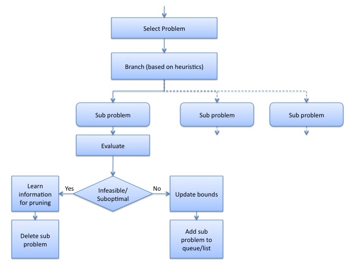
There are several ways to go about branch and bound search, which can be derived from the order in which the branching and bounding is done.

Status of a Subproblem:

• Generated: The subproblem is decomposed from a parent subproblem.
• Evaluated: An upper bound and a lower bound for the subproblem is defined by the information we have so far.
• Examined: Either a branching operation is performed on a subproblem, or the subproblem is pruned.

By specifying the corresponding operations on a subproblem in a specific status, we can define the order of processing each subproblem. Mainly there are two different order paradigms. (Assuming we are solving a minimization problem)

Iteration: Keep a variable to save the best upper bound we get so far, and a list containing all subproblems that are evaluated but not examined. At each iteration, we select the subproblem in the list with the smallest lower bound (the one with the smallest lower bound is more likely to find a minimal solution), and determine whether we should apply the branching operation or the elimination operation on it. The newly generated subproblem will be pushed into the list.

Advantage: The selection of the next subproblem is optimal, and we can have tighter bound to have shorter run time.

Disadvantage: We need a lot of space to store the list.

Iteration: Keep a variable to save the best upper bound we get so far, and a list containing some subproblems that are neither evaluated nor examined. At each iteration, if the last examined subproblem was decomposed, insert all children of the subproblem into the list, except the children that are evaluated and examined. If the last examined subproblem was eliminated, choose the newest subproblem in the list to evaluate and examine.

Advantage: The storage requirement is small. The child subproblem will be evaluated next to the parent subproblem, thus it can use the bounding information from the parent subproblem to speedup the evaluation operation. Feasible solutions are found quickly.

Disadvantage: It might generate a lot of subproblems in total, and requires more run time to solve all subproblems.

There are three main approaches to parallelize the branch-and-bound algorithm:

1. Operation-based parallelization: When we need to apply the same operation on several subproblems, we can do it in parallel. (Task parallelism/Data parallelism)
2. Structure-based parallelization: We can explore different branches (or solve different subproblems) in parallel. (Task parallelism)
3. Construction-based parallelization: By setting different constraints, we can construct several branch-and-bound trees at the same time (for example, by using different branching heuristics in each branch-and-bound tree) (Task parallelism)

For the operation-based approach, we need to collect a bunch of subproblems first, and apply the proper operations on them. Such synchronization slows down the performance of the algorithm. For the construction-based approach, it is possible that a lot of separate trees are solving the same subproblems. The duplication behavior makes this approach inefficient. Therefore, most research focuses on structure-based parallelism.

The structure-based parallelism can be classified into 4 categories:

1. Synchronous Single Pool (SSP): We synchronize all processors once in a while to update the best upper bound and lower bound information. Moreover, all processors share one pool, storing subproblems that need to be solved. (Shared queue)
2. Asynchronous Single Pool (ASP): We do not arbitrarily synchronize all processors. Processors will communicate on their own pace. All processors share one task pool. (Shared queue)
3. Synchronous Multiple Pool (SMP) : We synchronize all processors. Each processor has its own task pool, storing subproblems belong to it. (Distributed data)
4. Asynchronous Multiple Pool (AMP): We do not synchronize all processors. Each processor has its own task pool. (Distributed data)

For the synchronous method, there is trade-off between the amount of communication and the pruning efficiency. If we synchronize all processors frequently, the communication cost will be high. However, each processor will have the best upper bound and lower bound up to date, which helps pruning the subproblems within each processor significantly. If we do not synchronize them very often, the communication overhead is low. However, each processor might need to deal with more subproblems because of the poor bounds. For the asynchronous method, processors communicate when needed. For example, if a processor has found a better lower bound, it can broadcast such information to all other processors. However, if too much processors want to communicate at the same time, the resulting conflict might be serious, and the frequent interruption might degrade the overall performance. Therefore, the synchronous method is better when the update is frequent, and the asynchronous method is better when the update is not very often.

For the single pool data structure, each processor can have access to the shared data directly. No message passing is required. However, we need to take care of possible data race situation. Moreover, because of the limited memory bandwidth, usually the memory access on shared memory architecture is not very efficient. For the multiple pool data structure, the data required for each processor is stored locally. The accessing speed is faster, and no data race situation will occur. However, if we need to communicate among processors, explicit message passing is necessary. Therefore, if it is very often that we will update the bounds and distribute tasks, the single pool data structure is better. If such communication does not occur frequently, the multiple pool data structure is better.

There are two rule-of-thumbs regarding task assignment:

1. In order to achieve the highest efficiency, we need to use as many processors as we can and use them as soon as possible.
2. Avoid giving processors subproblems that have only a small chance of leading to an optimal solution. In other words, we will give processors subproblems that are more likely to prune more branches.

Some methods are proposed to achieve these goals:

• Use one processor to solve the original problem, and gradually broadcast among processors the units of tasks as they are created. (Master/worker)
• Use one processor to solve the original problem until the number of generated subproblems is enough. Then send these subproblems to other processors. (Master/worker)
• All the processors construct the same branch-and-bound tree. When the branching operation occurs, each processor select different subproblems to solve. (Actors)

For the first method, tasks are distributed frequently. Therefore, the idle processors can have tasks as soon as possible. However, the communicate overhead resulting from distributing tasks is high. For the second method, tasks are not distributed frequently. The communication cost of distributing tasks is low. However, it is possible that some of the processors will idle for a long time. Therefore, the first method is better while the tasks assigned for each processor is light-weight. The second method is better while the tasks assigned for each processor is computational intensive. For the third method, we do not need to distribute tasks among processors. However, the duplicate branch-and-bound tree in each processor might occupy a lot of memory. Moreover, we need to guarantee that no two processors are working on the same subproblems to prevent redundancy.

There are two ways to assign subproblems to processors:

1. Static assignment: A given number of subproblems are initially created, and processors subsequently solve these tasks.
2. Dynamic assignment:

• Assignment on request: A processor with an empty pool sends request for work to other processors. If the request is accepted, some tasks are transferred to the working pool.
• Assignment without request: Processors decide to share work units without being requested to by other processors.
• Combined assignment: Processors exchange tasks without being asked for, and send requests when their working pools are near empty.

For the static assignment method, once a processor has finished its job, it will idle until it is assigned new tasks. For the dynamic assignment method, if a processor is idle, it can find tasks by request or from the shared queue. The utilization rate of the processors will be higher. However, the communication cost of the dynamic assignment method is higher than the static method.

Precondition: The number of subproblems should be finite.

Invariant:

• For a minimization problem, a finite upper bound for any evaluated subproblem corresponds to a feasible solution to the original problem.
• For a maximization problem, a finite lower bound for any evaluated subproblem corresponds to a feasible solution to the original problem.
• For an optimization problem, a subproblem is solved if it is evaluated, and its upper bound equals its lower bound.

As a case study, consider the CNF-SAT satisfiability problem. The input to the problem is a set of clauses in the Conjunctive Normal form i.e Each of the clauses is a logical OR of one or more boolean variable or its complement. The objective is to find an assignment to all the variables so that each of the clauses evaluates to TRUE or report unsatisfiable if no such assignment exists.

The search space is the set of all possible assignments to the variables (Search space size = 2^n where n is the number of variables). The classical way to solve it is to assign a variable to a value (TRUE or FALSE)(branch) and see if this forces some other variables to particular values (from the constraint that all clauses must be satisfied). This is followed by another assignment until a satisfiable assignment is found or an unsatisfiable clause is found. If an unsatisfiable clause is found, then we conclude that the current search space is infeasible and add this information as a clause to the original problem. One of the assignments is flipped from TRUE to FALSE or vice versa (backtrack). Then the search procedure is continued till a solution is found or the entire space is found to the infeasible.

Another example is the traveling salesman problem (TSP). A TSP is that given n cities and the distance between any pair of cities, a traveling salesman is trying to find a cyclic path that visits each city once and has the shortest traveling distance. Given a traveling salesperson problem G=(V, E). |V| = n. We need to find the route with minimum cost. A path p is defined as a sequence of distinct nodes p={v1, v2, v3, …, vk}. Let c(p) denote the cost by walking along the path p. Let d(u, v) denote the minimum distance between u and v. A feasible solution can be defined as a n-tuple {x1, x2, x3, …xn}, if each xi represents a node, all elements in the tuple are distinct, and there is an edge from xi to x(i+1) 1⇐i⇐n-1, and from xn to x1. Given a path p with size less than n, we can define the subproblem as all possible routes starting with p. The branching operation can be formulated as: p={v1, v2, v3, …, vk}; the branches are p’1={v1, v2, v3, …, vk, u1}, p’2={v1, v2, v3, …, vk, u2}, …, p’n-k={v1, v2, v3, …, vk, un-k}, while u1, u2,…, un-k are all distinct from v1 to vk. Whenever we have got a feasible solution, we can update the global upper bound by the cost of the feasible solution. The lower bound of a subproblem on a path p can be defined as c(p)+d(vk, v1), while vk is the last element in the path, and v1 is the first element in the path.

The branch and bound pattern has been used to solve several search and optimization problems.

• Integer Linear Programming (ILP)
• Boolean Satisfiability (SAT)
• ESPRESSO family of logic optimization algorithms
• Automatic test pattern generation, such as PODEM

• Agent and Repository
• Task Parallelism
• Data Parallelism
• Graph Algorithms
• Shared Queue
• Distributed Data
• Master/Worker
• Actors

Bor-Yiing Su, Bryan Catanzaro, Narayanan Sundaram