Contents
Name
Monte Carlo Methods
Problem
The solution to some problems can be estimated by statistical sampling its solution space with a set of experiments using different parameter settings. How do we efficiently construct and execute thousands to millions of experiments, analyze the results, and arrive at a solution?
Context
How would you estimate the value of Pi experimentally? How would you estimate the expected profit from a trading strategy given various market conditions? Sometime, it is easy to solve a problem by setting up experiments to sample the solution space, but hard to solve the problem analytically.
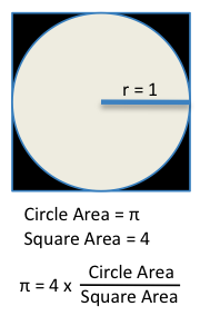
To estimate the value of Pi experimentally, we can throw darts at a square that is inscribed with a circle. We can estimate Pi by computing the ratio of the darts landed within the square vs the darts landed within the circle. Evaluating whether a particular dart landed within the circle is easy, evaluating Pi analytically is hard.
 To find the expected profit from a trading strategy, we try out the strategy over a variety of market scenarios in a set of experiments. We generate a market scenario based on the expected movement of the market with specific models of uncertainties. We then apply the strategy to the market scenario, simulating the decisions of the strategy over time. Applying the rules in the strategy during an experiment across time steps is easy, integrating the effects of all the rules analytically across time steps is hard.
By statistically sampling a problem’s solution space, we gain valuable insights into complex problems that are impossible or impractical to solve analytically. The quality of a solution estimated through sampling depend on several factors:
-
The statistical models used for sampling: parameters in the experiment may have irregular statistical variations that are hard to model analytically; using a realistic model is critical for the relevance and accuracy of the solution.
-
The coverage of the solution space: the approach assumes that experiments are independent and identically distributed (i.i.d.), such that the set of experiments provide a statistically significant sampling of the solution space
-
The statistical significance of solution: the statistical error in the solution is proportional to the inverse square-root of the experimental size, i.e. to achieve 10x more precision in the result, one need to run 100x experiments
The ease and intuitiveness of setting up the experiments make the Monte Carlo Method a popular approach. However, because of the large number of experiments required to achieve statistically significant solutions, it is extremely computationally intensive. Efficient execution of the experiments can make this method practical to a wide range of applications.
Forces
Universal forces:
-
Complexity of parameter modeling: we want to use as simple a statistical model as possible to model the parameter, simplicity leads to ease of understanding and programming, and allows for efficient computation; at the same time, the parameter model need to be detailed and complex enough to properly represent the statistical variations in the input parameters.
-
Speed vs statistical rigor in scenario modeling: we want to quickly generate many scenarios for experiments, at the same time, the scenarios generated must be independent and identically distributed based on properly sequences of random numbers to achieve the intended coverage of the solution space.
Implementation forces:
-
SIMD efficiency in packing experiments: we can give each experiment one thread, but one experiment may not be able to use all the parallelism of SIMD parallelism in a thread; on the other hand, we can give each experiments one SIMD lane, but execution traces may diverge between experiments, lowering SIMD efficiency.
-
Experiment data working set size: we can allow a single experiment to use each processor to be sure to have data working set fit in cache, but execution is exposed to long memory latency; we can allow multiple experiments to share a processor to hide long latency memory fetches, but the working set may not fit in limited cache space.
Solution
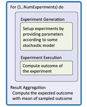 Solving a problem with the Monte Carlo method involves a sampling of the solution space with thousands to millions of experiments. The numbers of independent experiments provide significant parallel opportunities, which high performance computing (HPC) experts often call “embarrassingly parallel”. While this describes the ample parallelism opportunities, there are still many implementation decisions that need to be made for efficient execution. Each experiment requires a three-step process:
-
Experiment generation: generating a random set of input parameters for an experiment
-
Experiment execution: executing the experiment with its input parameter
-
Result aggregation: aggregating the experimental results to into statistical relevant solutions.
At the top level, we may have one problem to solve, or a set of problems to solve. In Pi estimation, we have one value to estimate; in option pricing, we often have a batch of thousands of options to price, where all options can be priced in parallel. When there is more than one problem to solve, we have the multiple levels of parallel opportunities to explore. Given the potential SIMD level and core level parallelism in the implementation platform.
Many problem specific tradeoffs can be made based on the execution behavior of the experiments. Map-Reduce Structural Pattern can be use here, where the problem is expressed as a two phase program with a phase-1 mapping a single function onto independent sets of data (i.e. sets of i.i.d. experimental parameters), and a phase-2 reducing the experimental results into a statistical estimation as a solution; the solution is composed of the efficient distribution and load balancing of the mapping phase, and efficiently collecting the results in the reducing phase.
In the next few paragraphs, we give an overview of the issues involved in sampling of the solution space in each of the three steps.
1. Experiment Generation
The experiment generation step involves setting up parameters for experiments to sample the solution space. The requirement for the Monte Carlo method is that the experiments are independent and identically distributed. We would like the parameters for the different experiments to be generated in parallel. This can be done, but one needs to be aware of the hidden states of generic random number generators (RNG) when they are producing sequences of random numbers. A typical RNG produces sequences of uniformly distributed random numbers. To model the parameters with various statistical properties, we need to convert a uniform distribution to the desired target distribution such as normal, lognormal distributions. The following subsections provide some guidelines for these two issues.
Random Number Generation
 There are two approaches to generating random numbers: one based on some physical phenomenon that is expected to be random, and the resulting numbers are often referred to “true” random numbers; the other uses computational methods to produce long sequences of apparently random results, usually determined by an initial value (or seed), where the generators are called pseudo random number generators.
For the purpose of this pattern, proper use of pseudorandom numbers is sufficient to generate independent and identically distributed sampling of the solution space. In software design, since reproducibility of sequences is invaluable for development, we will limit the discussion to pseudo random numbers and their generators.
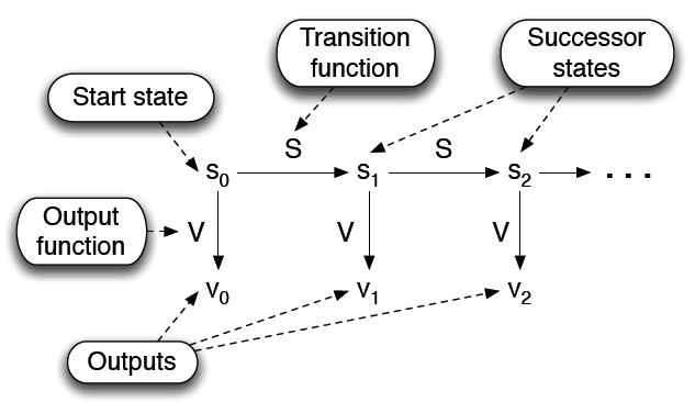
Pseudorandom numbers are generated using state machines with: a) a start state, b) a state transition function, and c) an output function.
The ISO C standard specifies that the rand() function provides a random sequence with a period of at least 232. This is often not large enough for experiment generation in Monte Carlo methods. To solve an option-pricing problem in computational finance, for example, it may require 16 variables per time step, a simulation scope of 1000 time steps, and the results of 1 million experiments to provide a result of the desired accuracy. To obtain independent and identically distributed experiments, it would require a sequence with a period of at least 234.
To resolve this issue, there exist special pseudo random generators such as the Mersenne Twister, which provides a period of (219937 − 1). The Mersenne Twister is derived from the fact that the period length is a Mersenne prime. The generator has an internal state of 624 32-bit integers. (Mersenne twister reference)
For a parallel execution, properly implementing a pseudo number generator faces further challenges. The pseudo random number generator random relies on internal states to produce the pseudo random sequence. In parallel processing, the internal state of a random number generator is a shared state between the different threads of computation, and can quickly become a performance bottleneck.
There are several approaches to resolving this bottleneck:
-
Pipeline the random number generation process: allow one of the processors to sequentially generate random number sequences in batches, to be consumed by other threads. (see PRNGlib reference)
-
Generate multiple unique sequences in parallel, using advanced parallel version of the Mersenne Twister PRNG or SPRNG Ver4.0, which have been proven to produce uncorrelated sequences when different choices of parameters are used.
Applying Statistical Models
The pseudo random generators usually produce uniformly distributed sequences, where as input parameters in Monte Carlo experiments may require a variety of statistical distribution. For example, the volatility of a stock in the market can be modeled with a lognormal distribution in its expected price; the performance of a computer circuit element affected by manufacturing process variation can be modeled by a normal distribution in its delay.
In performing the distribution conversion, it is important to provide an array of values to be converted at a time where possible, as many library routines are optimized to use SIMD instructions to efficiently take advantage of instruction level parallelism in processing an array of inputs.
There exist many of-the-shelf math libraries that are optimized for distribution conversion. One such example is the Intel Math Kernel Library (MKL). (Reference Intel MKL)
2. Experiment Execution
Statistical sampling the solution space with the Monte Carlo method involves running thousands to millions of independent experiments. This step is often perceived as the “Map” part of a MapReduce structural pattern. The experiments can be trivially mapped onto separate cores using Task Parallelism Strategy Pattern, where the problem is expressed as a collection of explicitly defined tasks, and the the solution is composed oftechniques to farm out and load balance the task on a set of parallel resources.
There is a more challenging aspect of parallelizing the experiments in SIMD lanes. The main performance issue here is with application specific program flow. The trade-offs are summarized in Table 1.
The experiments could have similar program flows, where instructions from multiple experiments can occur in lock step: the SIMD execution patterncan be applied here, where the problem is expressed as the challenge of efficiently executing instruction sequences in lock step across lanes (for multiple problems) to amortize instruction management overheads; and the solution is composed of efficient control flow and data structure to allow instruction fetch and data fetch overheads to be shared across SIMD lanes.
On the other hand, the experiments could have very different program flows, where experiments diverge into following different segments in the instruction stream. In which case we may have to look for parallelism within each experiment to take advantage the SIMD capabilities on modern multicore and manycore platforms.
The data working set of the experiments is also an important factor in achieving an efficient implementation. Modern multicore and manycore platforms provides limited fast memory close to the arithmetic units. Packing multiple experiments into SIMD lanes can significantly increase the amount of data (or operands) accessed. Even for moderately sized experiment working set, this can have sever cache efficiency implications. One can attempt to mitigate this problem by analyzing the access pattern of the experiment working set, storing more intermediate results in registers if possible, and where supported, designate some of the single-use data to be streaming.
Table 1. matrix of possible implementations
| Similar program flow | Divergent program flow | |
|---|---|---|
| Small data working set |
Pack multiple experiments into SIMD lanes. See SIMD Execution Pattern |
Look for SIMD parallelism within an experiment |
| Larger data working set |
Analyze working set Reduce cached working set Designate some operands to be streaming (not cached) |
Look for SIMD parallelism within an experiment |
3. Result Aggregation
The final solution of a statistical sampling of the solution space is the summarization of the individual experimental result. The results can be aggregated using the collective execution coordination pattern, where the problem is expressed as the challenge of efficiently summarize results from thousands to millions of locations, and the solutions is composed of logarithmically collecting the information in a tree form, leveraging the capabilities of the implementation platform.
The results and also be summarized to a fixed location as they are produced using atomic operations. In this case the Mutual Exclusion execution coordination pattern is used, where the problem is expressed as the challenge of updating a piece of memory (summary record) by one process/thread (experiment) at a time, and the solution is composed of software locks and semaphore, or explicit hardware support to manage the exclusivity of accesses/updates.
If the summarization function is associative, we can use collectives. One should note that we can only use atomic operations for summerization if the summarization function is commutative.
Invariant
Precondition: The system description is stateless and does not change by doing experiments on it.
Invariant: Experiments are independent and identically distributed to achieve statistically valid sampling.
Examples
Two examples are presented here:
-
Estimating Pi: illustration of the three steps, one problem to solve
-
Option Pricing: modeling input parameter distribution, many problems to solve
Estimating Pi
Estimate π by throwing darts at a square inscribed with a circle.
Calculate percentage that fall in the circle
Area of square = (2r)2 = 4
Area of circle = π r2 = π
-
Random number generation: Randomly throw darts at x,y positions, center of circle: x=0, y=0
-
Scenario Simulation: If x2 + y2 < 1, then point is inside circle
-
Result aggregation: π = 4 * # points inside / # points total
Option Pricing
We are trying to determine the present-day-value of a contract with this scenario:
“In 3 months’ time a buyer will have the option to purchase Microsoft Corp. shares from a seller at a price of $25 per share.”
The key point is that the buyer has the option to buy the shares. Three months from now, the buyer may check the market price and decide whether or not to exercise the option. The buyer would exercise the option if and only if the market price were greater than $25, in which case the buyer could immediately re-sell for an instant profit.
This deal has no downside for the buyer – three months from now the buyer either make a profit or walk away unscathed. The seller, on the other hand, has no potential gain and an unlimited potential loss. To compensate, there will be a cost for buyer to enter into the option contract. The buyer must pay the seller some money up front. The process in which we determine the cost of the up-front payment is the option-pricing problem.
In 1973, Robert C. Merton published a paper presenting a mathematical model, which can be used to calculate a rational price for trading options. (He later won a Nobel prize for his work.) In that same year, options were first traded in the open market.
Merton’s work expanded on that of two other researchers, Fischer Black and and Myron Scholes, and the pricing model became known as the Black-Scholes model. The model depends on a constant σ (Sigma), representing how volatile the market is for the given asset, as well as the continuously compounded interest rate r.
The Monte Carlo Method approach takes M number of trials as input, where M could be 1,000 to 1,000,000 large depending on the accuracy required for the result. The pseudo code for one individual experiment is shown below.
// A Sequential Monte Carlo simulation of the Black-Scholes model
1: for i = 0 to M − 1 do
2:    t := S · exp ((r − 0.5*σ^2)· T + σ√T · randomNumber())     ◃ t is a temporary value
3:    trials [ i ] := exp(−r · T ) · max{t − E, 0}
4: end for
5: mean := mean( trials )
6: stddev := stddev( trials , mean)
-
S : asset value function
-
E: exercise price
-
r: continuously compounded interest rate
-
σ: volatility of the asset
-
T : expiry time
-
M : number of trials
The pseudocode also uses several internal variables:
-
trials : array of size M , each element of which is an independent trial (iteration of the Black-Scholes Monte Carlo method)
-
mean: arithmetic mean of the M entries in the trials array
-
randomNumber(), when called, returns successive (pseudo)random numbers chosen from a Gaussian distribution.
-
mean(a) computes the arithmetic mean of the values in an array a
-
stddev(a, mu) computes the standard deviation of the values in an array a whose arithmetic mean is mu.
-
confwidth: width of confidence interval
-
confmin: lower bound of confidence interval
-
confmax: upper bound of confidence interval
Random Number Generation
In a parallel implementation, the computation in line (2-3) can be computed by concurrent threads of execution. The function randomNumber() must be generating uncorrelated (pseudo)random number sequences using components such as Mersenne Twister PRNG or SPRNG Ver4.0 for the concurrent threads of execution.
Scenario Simulation
The execution can be implemented to target multiple levels of parallelism in modern highly parallel execution.
Result Aggregation
Line (5-6) in the algorithm aggregates the results of the trials and provide a summary of the simulation results.
Known Uses
Many sources of the known uses are taken from wikipedia.
Physical sciences
Statistical physics
-
Goal:
-
Parameter:
-
Typical experiment size:
-
Available Packages
Molecular modeling
-
Goal:
-
Parameters:
-
Typical experiment size:
-
Available Packages:
Design and visuals
Global illumination computations
-
Goal:
-
Parameters:
-
Typical experiment size:
-
Available Packages:
Monte Carlo methods have also proven efficient in solving coupled integral differential equations of radiation fields and energy transport, and thus these methods have been used in global illumination computations which produce photorealistic images of virtual 3D models, with applications in video games, architecture, design, computer generated films, special effects in cinema.
Finance and business
Financial Risk Analysis
-
Goal: Simulating the effects of uncertain market conditions on the liability exposure of a contract or trading strategy
-
Parameters: Market conditions such as interest rates, prices of financial instruments (usually modeled by Brownian Motion with drift and volatility)
-
Typical experiment size: 5,000 to 500,000 experiments
-
Available Packages:
Telecommunications
Quality of service simulations – “Can you hear me now?”
-
Goal: Wireless network must be designed to handle a wide variety of scenarios depending on the number of users, their locations and the services they want to use. The network performance is evaluated with a Monte Carlo engine generating user states. If service levels are not satisfactory, the network design goes through an optimization process.
-
Parameters: user state (location, services used)
-
Typical experiment size: ?
Circuit Design
Statistical Timing analysis
-
Goal:
-
Parameters:
-
Typical experiment size:
-
Available Packages:
Related Patterns
-
MapReduce Structural Pattern: used for managing experiment execution and result aggregation steps
-
Task Parallelism Strategy Pattern: used for managing experiment execution
-
SIMD Execution Control Pattern: used for grouping experiment execution
-
Collective Execution Coordination Pattern: used for summarizing results
-
Mutual Exclusion Execution Coordination Pattern: used for summarizing results
References
-
M. Mascagni and A. Srinivasan, Algorithm 806: Sprng: A scalable library for pseudorandom number generation, ACM Transactions on Mathematical Software, 26 (2000), pp. 436–461.
-
N. Masuda and F. Zimmermann, PRNGlib: A Paral lel Random Number Generators library, Tech. Rep. CSCS-TR-96-08, Swiss National Supercomputing Centre, CH-6928 Manno, Switzerland, May 1996.
-
M. Matsumoto and T. Nishimura, Mersenne twister: A 623-dimensionally equidistributed uniform pseudo-random number generator, ACM Transactions on Modeling and Computer Simulation, 8 (1998), pp. 3–30.
-
F. Black and M. S. Scholes, The pricing of options and corporate liabilities, Journal of Political Economy, 81 (1973), pp. 637–654.
-
D. J. Higham, Black-Scholes for scientific computing students, Computing in Science and Engineering, 6 (2004), pp. 72–79.
-
R. C. Merton, Rational theory of option pricing, Bell Journal of Economics and Management Science, (1973).
Authors
Jike Chong