The problem involves updates to a system where each element of the system rigorously depends on the state of every other element of the system. How do we compute (or approximate) these updates in an efficient and scalable fashion?

This problem often occurs in the domain of natural sciences, where the objects with properties represent physical bodies or elementary particles that affect each other through physical forces stemming from gravity or electromagnetic field. The object’s instantaneous change in position, velocity, acceleration, and momentum can be computed based on positions and intrinsic properties such as mass or charge of all other particles in the system. Each iteration of such computation corresponds to a period in time. The users of the computation are typically interested in running this simulation in the time domain for some period of time or until some condition is met, such as achieving some steady state behavior. All or some intermediate time steps are typically of interest.

In a given iteration, object properties updates are independent of each other. The parallel implementation typically involves partitioning the objects between the PEs so that their properties can be updated concurrently. The pattern refers to the following term that we define as follows:

Object – an independent entity whose properties for the current iteration can be computed based on the properties of all objects in the previous iteration.

Property – an annotation of the object that has a value.

Distance – Measure of separation between the objects in a geographical space (usually the physical xyz co-ordinates, but could be more abstract)

Force – the interaction between the objects that changes the property (usually a decreasing function of the distance between the objects)

Slight variations on the pattern include cases where :

1. The interactions are between one set of objects and another i.e. each object in set A depends on all objects in set B.
2. Force is independent of distance (all objects affect equally)

Due to the often relatively light computational requirements of the properties update procedure, the computetocommunication ratio for each PE can be quite low. Therefore, the number of objects that are allocated to one PE has to be balanced carefully with communication. However,

1. When too many objects are allocated per PE, the computation may be unnecessarily serial, but the compute and communication will be better balanced.
2. When too few objects are allocated per PE, the computation is well parallelized, but will likely to be communication dominated. Also, if object updates require varying amounts of computational efforts, load balancing problems can easily arise.
3. Space partitioning needs to be done without destroying memory locality. Good locality implies objects closer in geographical space should reside closer in memory. This implies data movement overhead as the particles move (change location) due to the forces acting on them.

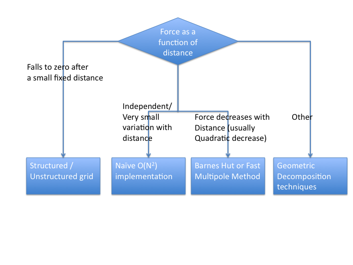
The following are some of the typical implementation strategies for Nbody interaction problem in physics. The approximation strategies, described below, benefit from particular properties of the force equations used to update the acceleration, velocities and positions of objects in space: the force equation is associative with respect to its inputs, the object positions. Before going into the details of specific implementation choices, the following flowchart might be needed to convince yourself that the N-body pattern really applies to the problem. If not, other related patterns that might be useful are Structured grid and geometric partitioning.

Naive algorithm – a straightforward O(n²) algorithm that simulates interaction of each object with every other object in the system. It is parallelized by evenly distributing the objects between processing elements. Each PE is responsible for updating only its objects. To do so, the PE receives object properties from all other PEs and uses them to perform the update. Then the PE sends the updated values to other PEs, and the process is repeated.

The exchange of object properties between PEs that happens between update iterations, cannot occur until all the PEs complete their updates. A typical Nbody computation waits on a barrier to ensure data consistency. The communication of the data between PE has to be carefully orchestrated to avoid overwhelming the communication fabric. One approach is to organize all PEs in a pipelined cycle, such that the data goes around the cycle to each PE, and enables each PE to perform necessary updates.

In absence of numerical problems and with sufficiently small time step, the Naive method returns the optimal numerical results.

The naive method will also have to be used in cases where the interactions between the particles cannot be assumed to decay with distance. In cases where it is not possible to approximate the interactions at large distances, the naive method is a good way of parallelizing the problem. For pseudo-code, refer to the example section of the pattern.

This O(n log n) approximation to the naive algorithm clusters the objects into “geographical” partitions and summarizes a partition in a way that enables distant objects to use the compact partition summary instead of detailed object properties. For example, a partition of objects far away (the distance to be determined by thresholds in the algorithm) can be summarized simply as a center of mass. This one quantity is used to update forces and positions of individual objects far away from this cluster center of mass.

The most important data structure for implementing Barnes-Hut is a quad-tree (2D) or oct-tree (3D). This refers to the partitioning of the particles in the geographical space. This partitioning could be static/dynamic. Even in the static case, it could be independent of the data(complete trees) or dependent on the distribution of the data (adaptive trees).

Figures: courtesy [4]

At a high level, the Barnes-Hut algorithm is as described below:

 1)  Build the Quadtree
 2)  For each subsquare in the quadtree, 
     compute the center of mass and total mass 
     for all the particles it contains.
 3)  For each particle, traverse the tree 
     to compute the force on it.

The second step of the algorithm is accomplished by a simple “post order traversal” of the quadtree (post order traversal means the children of a node are processed before the node). Note that the mass and center of mass of each tree node n are stored at n; this is important for the next step of the algorithm.

Given a list of particle positions, this quadtree can be constructed recursively as follows:

 procedure QuadtreeBuild
   Quadtree = {empty}
     For i = 1 to n          ... loop over all particles
       QuadInsert(i, root)   ... insert particle i in quadtree
     end for
     ... at this point, the quadtree may have some empty 
     ... leaves, whose siblings are not empty
     Traverse the tree (via, say, breadth first search), 
       eliminating empty leaves

 procedure QuadInsert(i,n)   
   ... Try to insert particle i at node n in quadtree
   ... By construction, each leaf will contain either 
   ... 1 or 0 particles
   if the subtree rooted at n contains more than 1 particle
      determine which child c of node n particle i lies in
        QuadInsert(i,c)
   else if the subtree rooted at n contains one particle 
      ... n is a leaf
      add n's four children to the Quadtree
      move the particle already in n into the child 
         in which it lies
      let c be child in which particle i lies
      QuadInsert(i,c)
   else if the subtree rooted at n is empty        
      ... n is a leaf 
      store particle i in node n
   endif

The pseudo-code for step 2 of the algorithm is as follows:

 ... Compute the center of mass and total mass 
 ... for particles in each subsquare
 ( mass, cm ) = Compute_Mass(root)   ... cm = center of mass

 function ( mass, cm ) = Compute_Mass(n)    
     ... Compute the mass and center of mass (cm) of 
     ... all the particles in the subtree rooted at n
     if n contains 1 particle
          ... the mass and cm of n are identical to 
          ... the particle's mass and position
          store ( mass, cm ) at n
          return ( mass, cm )
     else
          for all four children c(i) of n (i=1,2,3,4)
              ( mass(i), cm(i) ) = Compute_Mass(c(i))
          end for
          mass = mass(1) + mass(2) + mass(3) + mass(4) 
               ... the mass of a node is the sum of 
               ... the masses of the children
          cm = (  mass(1)*cm(1) + mass(2)*cm(2) 
                + mass(3)*cm(3) + mass(4)*cm(4)) / mass
               ... the cm of a node is a weighted sum of 
               ... the cm's of the children
          store ( mass, cm ) at n
          return ( mass, cm )
     end

The algorithm for step 3 of Barnes-Hut is as follows:

    ... For each particle, traverse the tree 
    ... to compute the force on it.
    For i = 1 to n
        f(i) = TreeForce(i,root)   
    end for

    function f = TreeForce(i,n)
        ... Compute gravitational force on particle i 
        ... due to all particles in the box at n
        f = 0
        if n contains one particle
            f = force computed using formula (*) above
        else 
            r = distance from particle i to 
                   center of mass of particles in n
            D = size of box n
            if D/r < theta
                compute f using formula (*) above
            else
                for all children c of n
                    f = f + TreeForce(i,c)
                end for
            end if
        end if

The correctness of the algorithm follows from the fact that the force from each part of the tree is accumulated in f recursively. [4]

This is a faster O(n), more accurate method. It differs from BarnesHut by computing potentials at every point (rather than forces), and by using a fixed set of boxes with more information rather than a varying number of boxes with fixed information.

A high-level description of FMM is as follows:

    (1) Build the quadtree containing all the points.
    (2) Traverse the quadtree from bottom to top, 
        computing Outer(n) for each square n in the tree.
    (3) Traverse the quadtree from top to bottom, 
        computing Inner(n) for each square in the tree.
    (4) For each leaf, add the contributions of nearest 
        neighbors and particles in the leaf to Inner(n)

Here, Outer(n) refers to the force created by particles inside square n to the outside of the square. Inner(n) refers to the force created by particles outside square n into it.

For more details, refer [5].

For the naive method, the most common parallelization strategy follows a pipeline pattern. Each PE/thread holds onto a few particles whose updates are controlled by it. In a pipeline fashion, other particles are passed from one PE to another (in a cycle) until each PE has updated its particles after interacting all other particles in the system. This is a strategy that works well and should be the first choice when implementing a parallel n-body problem using the o(N^2) method.

Load balancing is one of the most critical problems for hierarchical algorithms such as BarnesHut and Fast Multipole Method. First, distributing the objects among Processing Elements is nontrivial since the objects are partitioned based on their geographical location. Second, the objects change position over computation iterations, and thus it might be necessary to repartition and redistribute the objects among PEs.

When looking at the framework design, we could consider the following components provided by the programmer/user that enable implementation of the naive as well as hierarchical methods:

Partitioner Distributes the objects into hierarchical regions and creates a corresponding mapping to PEs. Partitioner communicates with the infrastructure to (1) specify PE mappings, and (2) conditions for infrastructure to force a repartitioning.

Summarizer Exports data from one hierarchical region to other regions. For example, in a naive algorithm, this would just export all the data, but a more sophisticated algorithm might export a summary: a center of mass and a force vector for objects in the region.

Local and nonlocal update procedures – Executed by PEs to combine properties of objects in this PE/hierarchical region with those in other PEs/regions.

There are other variations on the classic N-body (Particle-Particle) problem. Some of them include Particle-Mesh, Particle-Multiple-Mesh, Tree-Code-Particle-Mesh etc [3]. A very simple variation involves cases where the interactions are not between all elements of one set, but between every element of one set (A) to every element of another set (B). A naive implementation of this problem would be a O(NM) solution. Better strategies are possible, if every particle in one set is only influenced by a much small number of particles in set B. This approach also implies geographical partitioning strategies (similar to quad-trees, oct-trees etc) to reduce the computations. Ray tracing is an example of this kind of interaction between rays and objects in a scene.

Precondition: A set of uniform objects, and uniform interactions between them.

Invariants:

Each computation iteration preserves the number of objects in the system and their properties as required by their update procedure (equivalent to conservation of mass/energy/momentum)

Laws of interactions between the objects do not change for all iterations

Postconditions: All data has been updated for each iteration

For all the examples, we assume that we have N bodies each with mass m_i at position (x_i, y_i) and moving with a velocity (vx_i, vy_i). The force acting on the particles is gravitational i.e. force between bodies i and j is F(i,j) = G m_i m_j/r_i,j³ (x_i-x_j, y_i-y_j) where r_i,j = sqrt( (x_i-x_j)²+(y_i-y_j)²).

The objective is to simulate the movement of the bodies over a series of time with steps dt.

The code for executing one time step is given below:

Assume v(i) be the velocity of particle i at any time step. v(i) = ( (vx(i), vy(i) )

for i = 0:N-1

vx_new(i) = vy_new(i) = 0 
x_new(i)=y_new(i) = 0
for j=0:N-1 
  if(j != i) 
    (x(i),y(i)) = (x(i),y(i)) + v(i)*dt
    (vx_new(i), vy_new(i)) = (vx(i),vy(i)) + F(i,j)/m(i) * dt
  endif
(vx(i),vy(i)) = (vx_new(i),vy_new(i))
endfor

endfor

for i=0:N-1

(x(i), y(i)) = (x_new(i), y_new(i))
(vx(i),vy(i)) = (vx_new(i),vy_new(i))

endfor

Let there be M processors/threads, among which the N particles are divided. For sake of simplicity, assume that M divides N. Each processor has 2 arrays – one local for which each processor is responsible for updating the x,v values and another which is passed among the threads

NP = N/M
m_pass = m(threadId*NP:threadId*NP+NP-1)
x_pass = x(threadId*NP:threadId*NP+NP-1)
y_pass = y(threadId*NP:threadId*NP+NP-1)

for i= threadId*NP:threadId*NP+NP-1

vx_new(i) = vy_new(i) = 0 
x_new(i)=y_new(i) = 0

endfor

for k=1:M

for i= threadId*NP:threadId*NP+NP-1
  for j=0:NP-1 
    if(j != i) 
      F(i,j) = G*m(i)*m_pass(j)/r(i,j)^3 (x(i)-x_pass(j), y(i)-y_pass(j) )
      (x(i),y(i)) = (x(i),y(i)) + v(i)*dt
      (vx_new(i), vy_new(i)) = (vx(i),vy(i)) + F(i,j)/m(i) * dt
    endif
  endfor
  nextId = (threadId+1)modulo M
  m_pass = m(nextId*NP:nextId*NP+NP-1)
  x_pass = x(nextId*NP:nextId*NP+NP-1)
  y_pass = y(nextId*NP:nextId*NP+NP-1) 
endfor

endfor

for i=threadId*NP:threadId*NP+NP-1

(x(i), y(i)) = (x_new(i), y_new(i))
(vx(i),vy(i)) = (vx_new(i),vy_new(i))

endfor

Simulation of astronomical bodies under gravity : A collection of interacting masses in free space (no outside fields). The masses affect each other’s acceleration and thus velocity and position as described by the Universal Law of Gravitation. Given the initial positions and velocities of all objects in the system, the computation can update these parameters using the Law, one time step (iteration) at a time.

Other particle codes in physics

ParticleinCell is a related computation that effectively implements Nbody and grid like computations: objects interacting in a field.

The following PLPP patterns are related to Nbody Interactions pattern:

Dataflow/Pipeline – a naive O(n^2) implementation of the Nbody simulation can use a pipeline to exchange (essentially, rotate) the object properties between the PEs to orchestrate the n^2 matchings between the parameters that are used in the update procedure.

Data/Task Parallelism – each object can be updated independently

Geometric partitioning – the set of bodies has to partitioned between the PEs geometrically

Structured/Unstructured Grid – computational pattern that is useful if the interaction between particles is very local (zero after a small fixed distance)

[1] “Rapid Solution of Integral Equations of Classical Potential Theory”, V. Rokhlin, J. Comp. Phys. v. 60, 1985

[2] “A Fast Algorithm for Particle Simulations”, L. Greengard and V. Rokhlin, J. Comp. Phys. v. 73, 1987

[3] “N-Body / Particle Simulation Methods”, http://www.amara.com/papers/nbody.html – Has a good discussion of variants on n-body methods, including particle-mesh, particle-multiple-mesh, tree-code etc.

[4] “Fast Hierarchical Methods for the N-body Problem, Part 1”, http://www.cs.berkeley.edu/~demmel/cs267/lecture26/lecture26.html – Has a detailed discussion of Barnes Hut method

[5] “Fast Hierarchical Methods for the N-body Problem, Part 2”, http://www.cs.berkeley.edu/~demmel/cs267/lecture27/lecture27.html – Has a detailed discussion of Fast Multipole Method and parallelization for N-Body methods

Yury Markovsky, Erich Strohmaier

Edit 02/24 Narayanan Sundaram