Contents
Problem
Many problems appear with natural optimal substructures where by optimally solving a sequence of local problems, one can arrive at a globally optimal solution. There can also be significant parallelism in solving independent locally optimal solutions. How can we organize data and computation to efficiently arrive at the globally optimal solution?
Context
In many problems such as finding critical path in circuit timing analysis, finding most likely sequence of signals in a symbol state space, or finding minimum edit distance between two strings, the solution space is exponential with respect to input, i.e. one can concurrently check an exponential number of alternative solutions, and compare them to find the optimal solution to the problem.
By imposing a computation sequence based on the problem’s structure, one can reduce the amount of computation for some classes of these problems from exponential to polynomial run time. The computation order (or sequence) limits the amount of parallelism in the problem. However, for large inputs (on the order of thousands to billions of elements), exponential time algorithms are not computationally practical. Polynomial time algorithms leverage problem structure to restrict computation sequence and avoid exponential computation.
There are two ways to compute the global optimal solution: top‐down and bottom‐ up. The top‐down approach starts from the top‐level problem and recursively divides the problem into a set of sub problems until it hits the smallest sub problem that it could solve trivially. The higher‐level problem obtains optimal solutions form its sub problems in order to produce a higher‐level optimal solution. In contrast, the bottom‐up approach does not have the recursive problem dividing phase; it simply starts from the smallest sub problem and provides the result up to the higher‐level problem. The top‐down approach should involve memoization to avoid redundant computations.
The parallel opportunities in this pattern is similar to the Divide‐and‐Conquer pattern with the following three properties: 1) there are natural initial division boundaries in the problem; 2) there are frequent, and well defined reduction and synchronization points in the algorithm; and 3) number of fan‐ins are strictly limited by the problem.
The two main difference compared to the Divide‐and‐Conquer pattern is: 1) the presence of overlapping shared sub‐problems, and 2) exponential size of the overall problem, which prohibits starting with the problem as a whole and then apply the divide‐and‐conquer techniques. In this pattern, the starting point is often the naturally defined set of sub‐problems, and computation is often limited to a wave‐ front of sub‐problems.
However, finding an efficient recursive relation of the problem may be non‐trivial. If this is the case try to express the problem using the Divide‐and‐Conquer pattern or Backtrack, Branch‐and‐Bound pattern first.
Forces
• Inherent forces (regardless to the implementation platform)
- Top-down or Bottom-up. Compared to the bottom‐up approach the top‐down approach has some overheads which are: (1) recursively splitting the top‐level problem into a set of sub problems, (2) function call overheads associated with recursion, and (3) a lot of redundant computation without memoization. The top‐down approach, however, might be a more natural way to think how the sub‐problems should be merged into a higher‐level optimal solution compared to the bottom‐up approach.
- Task granularity. To increase the amount of parallelism in the problem, we want smaller sub‐problems that can be independently processed. However, the frequent reduction of limited scope pushes for more local reductions to take place within a task to avoid task‐to‐ task synchronization cost.
• Implementation forces
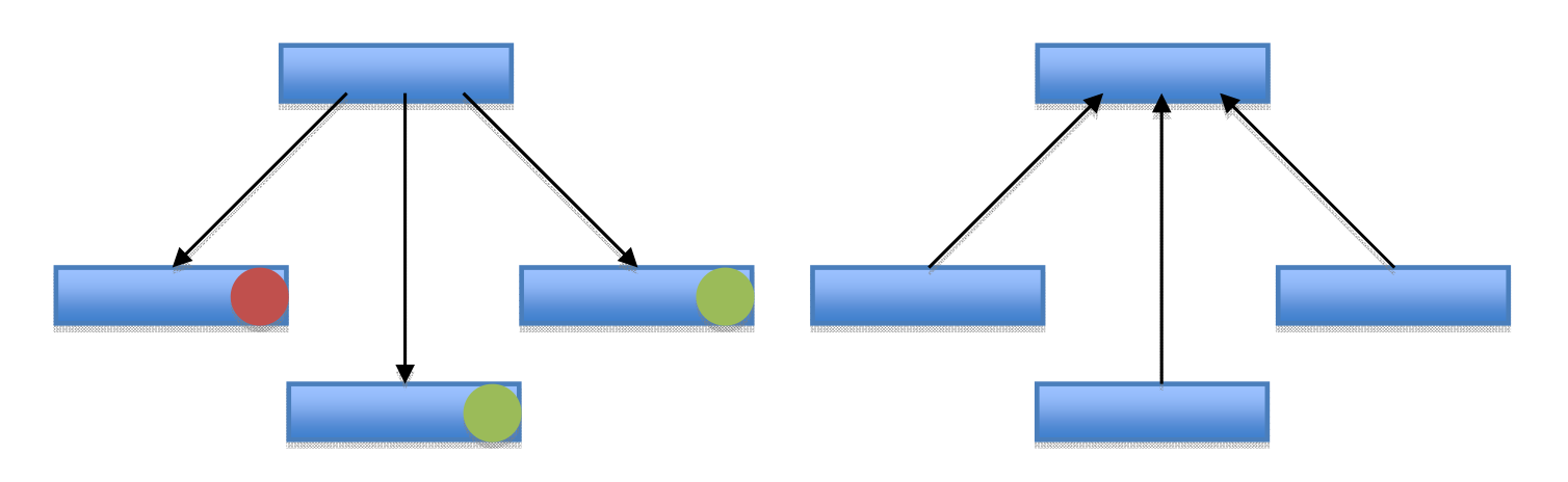
- Push or pull reduction. The restriction on computation order requires the synchronization between sub‐problems. When computing a local or a global optimal solution on the parent, the parent can pull the results from its children, or the child can push the results to parents. Normally when the parent is pulling the results from the children, each child has some local storage to save the result until the parent decided to read the result. Pulling by the parent involves polling on the state of the results from its children, which could block the parent from doing other useful work. In contrast, when the children are pushing the result to the parent, it doesn’t involve any local storage, because the child is “pushing out” the result. Though pushing by the children could cause contention problem at the parent, as the children of the parent could be all producing results, and pushing concurrently. The left figure represents a pull situation. The parent polls the children whether it have finished its computation. The red light means that the child node is still computing, the green light means that the child node is done and represents the local data, which is the optimal solution for the children. The right figure explains a push situation. Right after the child finishes its computation, it pushes the result to the parent. The child might involve any atomic computations.
- Reduction synchronization scope. The synchronization between parent and child could be across an entire level of sub‐problems to amortize synchronization overhead, but such solutions require good load balancing at each level. On the other hand, the reductions could involve individual locks on each sub‐problem, which is sensitive to efficiency of atomic action implementation on a platform.
- Data layout. For data locality of solving the sub‐problems, data associated with each sub‐problem should be distributed to each sub‐ problem. However, data such as parameter lookup tables should be shared among many sub‐problems to save storage, which also makes it easier to manage stored centrally.
Solution
(1) Find a recursive relation. If you are already have your recursive relation, go to the implementation stage which starts from (4). Read the problem carefully, and find out if you could divide the problem into sub‐problems. The most important thing for the dynamic programming pattern is that you should prove that the solution of the higher‐level problem expressed in optimal solutions of the sub‐ problems is optimal. This part might be tough; if you can’t figure out a recursive relation, try the divide‐and‐conquer pattern or the backtrack, branch‐and‐bound pattern. By doing that you might find a recursive relation between sub‐problems.
(2) What is the answer of the problem? Now express your global optimal solution in terms of the recursive relation that you found in the previous stage (1).
(3) Try an example to verify the recursive relation. You might have got the recursive relation wrong. Try a simple example by walking through the recursion, and do the math. You would get an insight whether your relation is right or wrong.
(4) Express the recursive relation topdown. Write down code that executes the recursive relation that you have found. First write down the trivial cases (i.e. boundary cases), and then make the top level function using the previous function.
(5) Use memoization to eliminate redundancy. After writing down the recursion, you will see that the program is doing the same computation over and over again. Introduce an array that saves the intermediate results. First search the array, and if the value is already there return that value, if not, enter the recursive function to calculate the solution.
(6) Express the recursive relation bottomup. The top‐down approach divides the problem top to bottom, and after hitting the trivial cases (i.e., boundary cases) it climbs up the ladder. The bottom‐up approach starts from the trivial cases and goes up. By writing a bottom‐up approach, you basically save the overhead of function calls. This might be the fastest version among your three versions of code.
(7) Parallelize. Even you did up to (6) and it takes too long to compute the global optimal solution, you have two choices. 1) Find a more efficient recursive relation in terms of time complexity which starts from step (1), or 2) parallelize your program.
There are three types of Solve and Reduce problems that require difference emphasis on solution approaches:
i. Input specific problem structure (e.g. circuit timing analysis)
In problems such as circuit timing analysis, the structure of the problem is problem instance specific. For each circuit, the structure of the sub‐problem corresponds to the structure of the circuit. The key parallelization challenge is to discover parallelism in the structure, partition and load balance the Units of Execution (UEs) at runtime.
The execution sequence constraints are usually trivially derived from the problem structure. To increase computation granularity, blocks of sub‐ problems are computed in serial in UE. These blocks could be discovered by lookahead of a few levels sub‐problems or by global partitioning on the entire set of the sub‐problems. Since the problem defines the number of in‐ degree of the sub‐problems, one can allocate distinct memory for storing sub‐problem solutions, such that each child can push its result to its parent without memory conflict. (Note: care must be taken with memory allocation of the result container, as memory location in the same cache line may still experience false sharing.)
In the circuit‐timing example, the longest path seen so far at each gate, including gate and wire delays can be accumulated, and pushed onto the fan‐in of the next gate. The reduction can occur at the granularity of individual blocks of execution. Natural data layouts for this type of problems usually involve a graph container with adjacency list representation storing the problem structure. Parallel graph partitioning techniques discussed in the Graph Traversal pattern can be used to increase the amount of parallelism in problem.
ii. Fixed problem structure (small fan‐in, independent local sub‐problems, e.g. string edit distance)For problems with fixed structure, communication and computation can be optimized at compile time. The key parallelization problem here is to find the optimal granularity, balance computation and communication, and reduce synchronization overhead.
The optimal UE granularity can be determined by autotuning for register/cache size and memory prefetch capabilities for a particular platform. Ghost cells can be used around a partition to bundle communications between UE to amortize overhead.
The existence of regular structures can allow interchanging phases of load balanced computation and communication to take place, such that results of sub‐problems can be pulled by the parents after a global barrier. The techniques used are very similar to those of Structured Grid pattern.
iii. Fixed problem structure (large fan‐in, inter‐dependent sub‐problems, e.g. Viterbi algorithm on trellis)Sometime the algorithm requires entire levels of sub‐problems to be solved, where all sub‐problems at each level depends on the solution of the previous level. Viterbi algorithm for finding the most likely sequence in a symbol space is an example. In this case, the problem constraints naturally imply the use of barrier between iteration for synchronization.
The key parallelization challenge is to efficiently handle the special all‐to‐all reduction in each iteration where the transition edges may carry different weights. Typically, there will be some default edge weights, but a significant portion of the edges that will have unique weights. The solution often calls for sink‐indexed adjacency‐list sparse representation for transition edges data layout. Sink‐index allows the current iteration to efficiently pull results from previous iteration, and the adjacency‐list sparse representation allow the use of Sparse Matrix pattern techniques for parallelization.
Invariant
- Precondition. The problem has a provable optimal substructure, which can be used to get a globally optimal solution
- Invariant. Locally optimal solutions are computed in the order defined by the structure of the problem to lead to a globally optimal solution
- Postcondition. The globally optimal solution is found.
Example
To take a closer look at the dynamic programming pattern, we describe some examples that encounter various forces.
- Fibonacci number
- Longest common Subsequence (LCS)
- Unbounded knapsack problem
- Shortest Path (Floyd–Warshall algorithm)
1. Fibonacci number
Problem. The following recursive relations define the Fibonacci numbers:
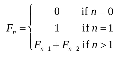
For a given n what would is the Fibonacci number Fn?
(1) Find the recursive relation. By definition, we could recursively call Fn‐1 and Fn‐ 2 in order to compute Fn. We only need to take care of the corner cases that are the cases when n is 0 or 1. The relation is, of course:

(2) What is the answer of the problem? The answer would be F (n).
(3) Try an example to verify the recursive relation. Let’s calculate F(5).
F(5) = F (4) + F(3) = 3 + 2 = 5
F(4) = F (3) + F(2) = 2 + 1 = 3
F(3) = F (2) + F(1) = 1+ 1 = 2
F(2) = F (1) + F(0) = 1+ 0 = 1
(4) Express the recursive relation topdown.
function fib(n) begin
    if n = 0 then return 0
        else if n = 1 then return 1
        else return fib(n-1) + fib(n-2)
end
Let’s take a look at the call graph of fib(5).
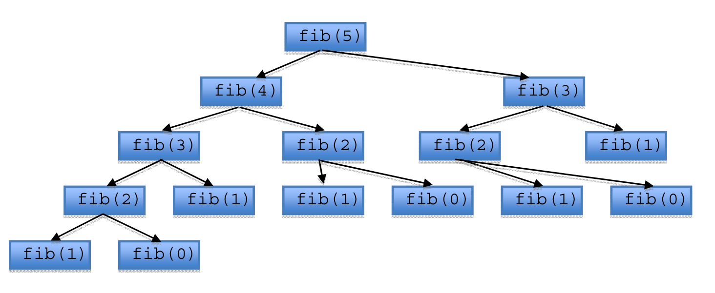
As you can see it evaluates fib(5) in a top‐down way. However, when n is greater than 1 fib(n) calls fib(n-1) and fib(n-2) consecutively. Even worse, there are redundant calls for fib(3) and fib(2). You could save the previous result of fib(n) and use it in the future. This technique is called memoization, it could benefit your code from an exponential time algorithm to a polynomial time algorithm
(5) Use memoization to eliminate redundancy.
var m = {0, 1, -1, -1, …}
function fib(n) begin
    if m[n] = -1 then m[n] = fib(n-1) + fib(n-2)
    return m[n]
end
Now the call graph of fib(5) looks like the following. The memoization technique saves the intermediate Fibonacci numbers while calculating, resulting fewer fib(n) calls.

(6) Express the recursive relation bottom-up.
function fib(n) begin
    if n = 0 then return 0
    else if n = 1 then return 1
    else begin
        var f = {0, 1, …}
        for i = 2 to n begin
            f[i] = f[i-1] + f[i-2]
        end
        return f[n]
    end
end
The bottom‐up version fills up an array from the bottom (i.e. fib(0), fib(1)) to the top (i.e. fib(n)). The Fibonacci number example describes different approaches for the dynamic programming pattern; a top‐down approach using divide‐and‐conquer with and without memoization and a bottom‐up approach.
(7) Parallelize. Let’s use the top‐down expressed Fibonacci implementation in (4). We could use the push method or pull method to communicate between the parent and the child. Let’s start with the push method. The first version is expressed in Clik. The second version is expressed using atomic add, and thread primitives.
function fib(n) begin
    if n = 0 then return 0
    else if n = 1 then return 1
    else begin
        value = spawn(fib(n-1)) + spawn(fib(n-2)) sync
        return value
    end
end
function fib(value, n) begin // value is call by reference
var local = 0
if n = 0 then begin
local = 0
end
else if n = 1 then begin
local = 1
end
else begin
create thread fib(local, n-1) as t1
create thread fib(local, n-2) as t2
join t1, t2
end
atomicadd(value, local)
endIf it were expressed in a pull fashion, it would look like the following. It defines a flag that the parent could poll to check whether the child has completed its computation or not. Each child has its local storage to store the computation result that the parent could read in the future.
function fib(n) begin
    if n = 0 then begin
        local storage = 0
        mark completed flag
    end
    else if n = 1 then begin
        local storage = 1
        mark completed flag
    end
    else begin
        create thread fib(n-1) as t1
        create thread fib(n-2) as t2
        poll completed flag of t1 and t2
        local store = local store of t1 + local store of t2
        mark completed flag
     end
end
2. Longest common subsequence (LCS)
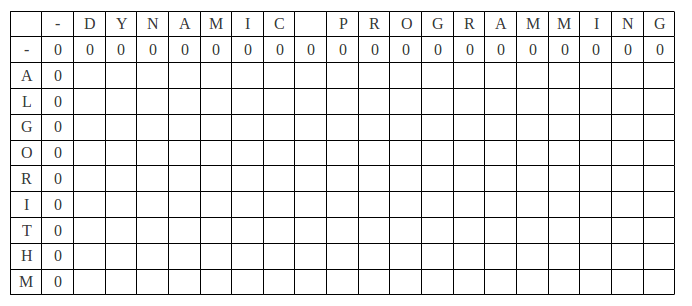
Problem. Find the longest subsequence common to all sequences in two sets of sequences. If the two set were “DYNAMIC PROGRAMMING” and “ALGORITHM” the longest common subsequence is “AORI”.
(1) Find the recursive relation. Let two sequences be defined as the following:
a = (a1, a2, …, ax)
b = (b1, b2, …, by)
We could define the recursive relation by:
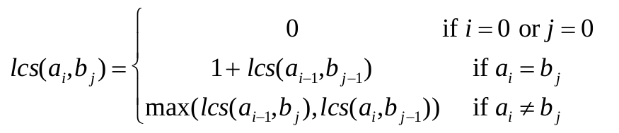
(2) What is the answer of the problem? The answer would be lcs(ax ,by ).
(3) Try an example to verify the recursive relation. Here is initial layout of array c.
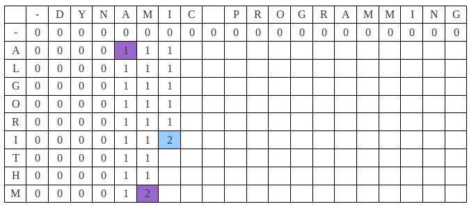
After a couple of iterations the table looks like the following. Now it is the turn to fill the blue colored cell. a[i‐1] and b[j‐1] are the same alphabet ‘I’ so the blue cell is filled with 1+c[i‐1, j‐1] which is “2”.
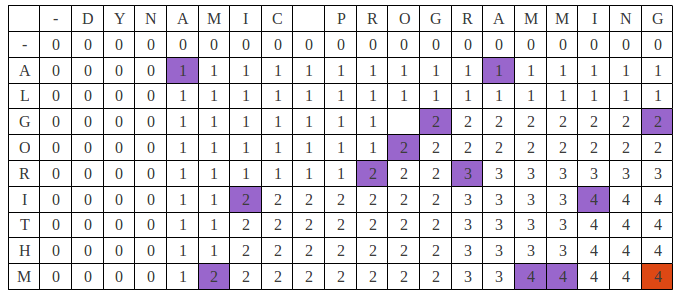
Finally, the table looks like this. Our optimal solution is “4” (the red colored cell).
(4) Express the recursive relation top-down.
function lcs(a, b) begin
    lcsr(a, b, 0, 0)
end

function lcsr(a, b, i, j) begin
    if a[i] = null or b[j] = null then return 0
    else if a[i] = b[j] then return 1 + lcsr(i+1, j+1)
    else return max(lcsr(i+1, j), lcsr(i, j+1))
end
(5) Use memoization to eliminate redundancy.
function lcs(a, b) begin
    lcsr(a, b, 0, 0)
end

var m = 2D array (size of first set * size of second set) initialized to -1

function lcsr(a, b, i, j) begin
    if m[i, j] = -1 then
        if a[i] = null or b[j] = null then m[i, j] = 0
        else if a[i] = b[j] then m[i, j] = 1 + lcsr(i+1, j+1)
        else m[i, j] = max(lcsr(i+1, j), lcsr(i, j+1))
    end
    return m[i,j]
end
(6) Express the recursive relation bottom-up.
function lcs(a, b) begin
    var x = size of first set
    var y = size of second set
    var c = 2D array (x * y) initialized to 0
    for i = 1 to x begin
        for j = 1 to y begin
            if a[i-1] = b[j-1] then
                c[i, j] = 1 + c[i-1, j-1]
            else
                c[i, j] = max(c[i-1, j], c[i, j-1])
            end
        end
    end
    return c[x,y]
end
(7) Parallelize. Similar to “1. Fibonacci Number” parallelize strategy.
3. Unbounded knapsack problem
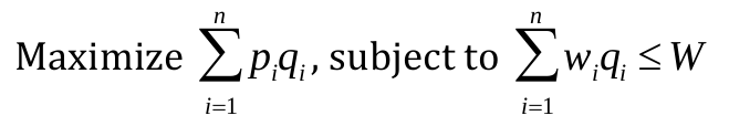
Problem. Let’s assume that we have n kinds of items and name then 1 through n. Each kind of item i has a value pi and a weight wi. We have a bag that could carry W max. The quantity of each items are unbounded. The challenge is to maximize the value of items that we could carry using the bag.
If we use qi to indicate the quantity of each item, the problem could be rephrased as following:
(1) Find the recursive relation. Let’s assume that V (w) indicates the maximum value of items that could be selected given a W size bag. The recursive relation could be written as:
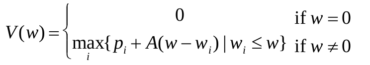
(2) What is the answer of the problem? The answer of the problem would be V (W ).
(3) Try an example to verify the recursive relation. Assume that we have five items. The value and weight of the items and the capacity of the bag are:
( pi,wi )=(1,1), (2,2), (2,3), (10,4), (4,12)
W =15
The initial state of V would be:
| W |
0 |
1 |
2 |
3 |
4 |
5 |
6 |
7 |
8 |
9 |
10 | 11 | 12 | 13 | 14 | 15 |
|
V |
0 |
‐1 | ‐1 | ‐1 | ‐1 | ‐1 | ‐1 | ‐1 | ‐1 | ‐1 | ‐1 | ‐1 | ‐1 | ‐1 | ‐1 | ‐1 |
The final state of V would be the following. Our optimal solution is “33”.
| W |
0 |
1 |
2 |
3 |
4 |
5 |
6 |
7 |
8 |
9 |
10 | 11 | 12 | 13 | 14 | 15 |
|
V |
0 |
1 |
2 |
3 |
10 | 11 | 12 | 13 | 20 | 21 | 22 | 23 | 30 | 31 | 32 | 33 |
(4) Express the recursive relation topdown.
function knapsack(p, w, n, W) begin
    var max = 0
    for cw = 1 to W begin
        var value = knapsackr(p, w, n, cw)
        if max < value then max = value
    end
    return max
end

function knapsackr(p, w, n, W) begin
    if W = 0 then return 0
    var max = 0
    for i = 1 to n begin
        if w[i] <= W then begin
            var value = p[i] + knapsackr(p, w, n, W-w[i])
            if max < value then max = value
        end
    end
    return max
end
(5) Use memoization to eliminate redundancy. In order to leverage memoization, we need to keep track of V (W ) .
function knapsack(p, w, n, W) begin
    var max = 0
    for cw = 1 to W begin
        var value = knapsackr(p, w, n, cw)
        if max < value then max = value
    end
    return max
end

var m = {0, -1, -1, …}
function knapsackr(p, w, n, W) begin
    if m[W] = -1 then begin
        var max = 0
        for i = 1 to n begin
            if w[i] <= W then begin
                var value = p[i] + knapsackr(p, w, n, W-w)
                if max < value then max = value
            end
        end
        m[W] = max
    end
    return m[W]
end
(6) Express the recursive relation bottom-up.
function knapsack(p, w, n, W) begin
    var V = {0, -1, -1, …}
    var gmax = 0

    for cw = 1 to W begin var
        max = 0
        for i = 1 to n begin
            if w[i] <= cw then begin
                var value = p[i] + V[cw-w[i]]
                if max < value then max = value
            end
        end
       V[cw] = max
       if gmax < V[cw] then gmax = V[cw]
    end
    return gmax
end
(7) Parallelize. Similar to “1. Fibonacci Number” parallelize strategy.
4. Shortest Path (Floyd–Warshall algorithm)
Problem. Given a graph G=(V, E), solve all‐pairs shortest‐paths. Let’s assume V = {1, 2, …, n}, and the weight between vertex i and j to be w(i, j) .
(1) Find the recursive relation. In order to figure out the recursive relations let’s consider a subset {1, 2, …, k} of vertices. D(i, j)k indicates the shortest path from i to j with all intermediate vertices in the set {1, 2, …, k}. We could develop our recursive relation by the following:
![]()
(2) What is the answer of the problem? Because all intermediate vertices in any path should be in the set {1, 2, …, n}, the answer of the problem all‐pairs shortest‐ paths should be the matrix Dn .
(3) Try an example to verify the recursive relation. Let’s assume our graph G=(V,E) is the following. V={1, 2, 3, 4, 5}, E is expressed in w(i, j) ‐ ∞ means no edge between vertex i and j. This example is from the “Introduction to Algorithms” book.
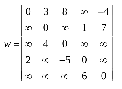
Here’s some intermediate Dk s.

Our final answer for the problem would be D5.
(4) Express the recursive relation top-down. This step is quite straightforward.
function floydwarshall(w, n) begin
    var D = 2D array (n * n)
    for i = 1 to n begin
        for j = 1 to n begin
            D[i, j] = fwr(w, n, i, j)
        end
    end
    return D
end

function fwr(w, k, i, j) begin
    if k = 0 then return w[i, j]
    else begin
        var c1 = fwr(w, k-1, i, j)
        var c2 = fwr(w, k-1, i, k) + fwr(w, k-1, k, j)
        return min(c1, c2)
    end
end
(5) Use memoization to eliminate redundancy. The thing to keep track is the intermediate results of fwr. We assign a 2D array to store the results.
function floydwarshall(w, n) begin
    var D = 2D array (n * n)
    for i = 1 to n begin
        for j = 1 to n begin
            D[i, j] = fwr(w, n, i, j)
        end
    end
    return D
end

var m = 3D array (n*n*n) initialized to infinity
function fwr(w, k, i, j) begin
    if m[k, i, j] = infinity then begin
        if k = 0 then m[k, i, j] = w[i, j]
        else begin
            var c1 = fwr(w, k-1, i, j)
            var c2 = fwr(w, k-1, i, k) + fwr(w, k-1, k, j)
            m[k, i, j] = min(c1, c2)
        end
    end
    return m[k, i, j]
end
(6) Express the recursive relation bottom-up. We could start from k=0 and increase k by filling the intermediate results bottom‐up.
function floydwarshall(w, n) begin
    var D = 3D array (n*n*n) initialized to infinity
    for i = 1 to n begin
        for j = 1 to n begin
            D[0, i, j] = w[i, j]
        end
    end
    for k = 1 to n begin
        for i = 1 to n begin
            for j = 1 to n begin
                var c1 = D[k-1, i, j]
                var c2 = D[k-1, i, k] + D[k-1, k, j]
                D[k, i, j] = min(c1, c2)
            end
        end
    end
    return D[n]
end
(7) Parallelize. Similar to “1. Fibonacci Number” parallelize strategy.
Known Uses
- Logic optimization: where circuit timing analysis is used as a sensor on how optimal the circuit timing is.
- Spelling check: uses the Levenshtein distance to check for correct spelling, and offer possible intended words that are closest to a misspelled word.
- Speech recognition uses Viterbi algorithm to match a sequence sound observation frame to a dictionary of known word pronunciations.
Related Patterns
- Divide‐and‐Conquer
- Backtrack, Branch and Bound
- Graph Traversal
- Structured Grid
- Sparse Matrix
References
- Introduction to Algorithms, second edition.
- Cilk 5.4.6 Reference Manual
- http://en.wikipedia.org/wiki/Dynamic_programming
- http://en.wikipedia.org/wiki/Fibonacci_number
- http://en.wikipedia.org/wiki/Longest_common_subsequence_problem
- http://www.ics.uci.edu/~eppstein/161/960229.html
- http://en.wikipedia.org/wiki/Knapsack_problem
Authors
- Original Author: Jike Chong, Youngmin Yi
- Revised 2/11/09: Yunsup Lee