Contents
Problem
Some Ordinary and Partial Differential Equations are easier to solve numerically after chang- ing the basis of the data representation. How do we perform these transformations in parallel?
Context
In the pattern language, “Spectral Methods” (SMs) appears mid-way through the sequence: after the developer has a mathematical understanding of the problem and can formulate the correct Ordinary Differential Equations (ODEs) or Partial Differential Equations (PDEs). SM is one of several methods of obtaining numerical solutions to such problems.
There are three primary motivations for using Spectral Methods. First, the approxima- tions provided by Fourier and Chebyshev series expansions are “exponentially convergent”. That is, if a length N expansion is used, the error in the approximation is O( (1/N)^N ), and thus can be used to provide many digits of precision. Second, since the high numerical accuracy of spectral methods reduces the number of grid points required to achieve precision, spectral codes can require less memory than other methods. This “memory-minimizing” property can be crucial, since a large memory footprint can, in the best case, cause a program to run slowly, and in the worst case cause the program to exhaust the memory capacity of the machine. Finally, Fourier-Spectral algorithms built on top of the Fast Fourier Transform or similar Divide-and-Conquer transformation algorithms can be implemented very efficiently. The serial operations count of such algorithms is within a factor of lg N (where N is the number of variables in the system) of the theoretical lower-bound.
The natural basis of representation for a problem is usually in terms of variables with immediate physical significance, for example spatial coordinates, time, density, temperature, and velocity. Other methods exist for solving the problem directly in terms of these variables. The simplest of these, for example, is the Forward Euler Method, which solves ODEs by repeatedly applying the formula yn+1 = yn + h · f (xn, yn), xn+1 = xn + h. The function f , which computes the derivative of y, is applied to the current values of the variables x and y at step n of the iteration. This method is undesirable because the error of the updated value is proportional to h2, the square of the increment applied to x. While simple to program, the tendency towards divergence places severe restrictions on how large a timestep one can use and makes the method impractical. Other methods exist which maintain the natural data representation, are more numerically stable than the na¨ıve Euler iteration, and are simpler to program than SMs.
The alternative that SMs provide is to approximate the functions of interest as series expansions in terms of a selected set of “basis functions”, that is:
![]()
The most useful expansions are the Fourier series and the Chebyshev series. In a Fourier expansion, the basis functions φ are the trigonometric functions sin(nx )an dcos(nx). If the function y(x) is complex-valued, the exponential eιx is used, where ι = √-1. The Chebyshev expansion uses the Chebyshev polynomials Tn(x) as the basis functions, where Tn(x) is defined by the following recurrence:
T0(x) ≡ 1,T1(x )≡ x
Tn+1(x) = 2xTn(x )− Tn−1(x)
By a change of variables, however, the Chebyshev polynomials can be made to be a trigono- metric function:
Tn(cosθ) ≡ cos(nθ)
Therefore, a Chebyshev series is really just a Fourier cosine expansion with a change of variable. For the purposes of this pattern, we focus primarily on the implementation of the Fourier expansions. Other choices of basis functions are Hermite Polynomials, Laguerre functions, Legendre Polynomials, and Gegenbaur Polynomials. The reader should consult a more specialized source for these techniques, although the Fourier and Chebyshev bases discussed above will suffice for nearly all applications. The Fourier series are directly applicable whenever the problem is periodic, or defined on a finite domain so that a periodic solution is appropriate. The Chebyshev series apply for non-periodic functions, but may require explicit boundary condition constraints.
Forces
The strided-neighbor “butterfly” communication patterns typically exhibited by functional transforms requires careful attention to data layout and movement. Machine characteristics require balancing of the size and number of inter-processor messages.
Solution
Note: The images here and much of the material are due to Jim Demmel and Rajesh Nishtala.
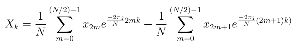
The implementation of a Fast Fourier Transform (FFT) is based on a recursive, divide- and-conquer formulation of the Discrete Fourier Transform. The most commonly used is the Cooley-Tukey:
Finally, in order for a parallel implementation to run efficiently, the individual sequential per processor implementations used as building blocks must run efficiently. There are several high-performance libraries that generate code for serial or low-degree parallel transforms: FFTW (the Fastest Fourier Transform in the West) and SPIRAL are two notable examples.
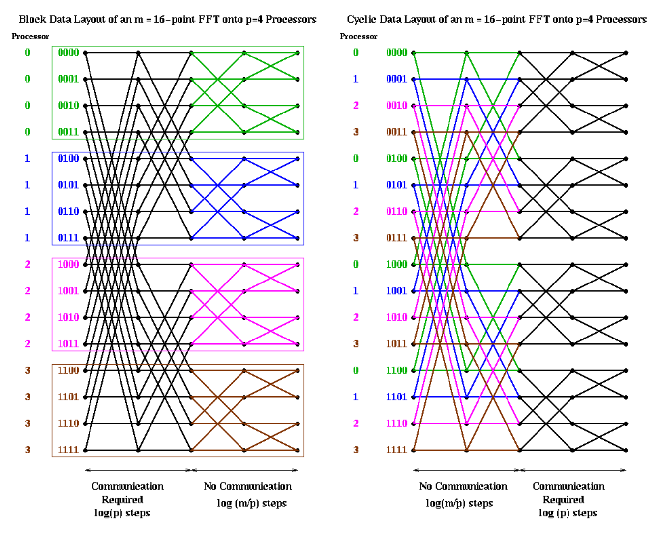
The computation within a 1-dimensional Cooley-Tukey FFT is highly data-parallel, but potentially requires an un-reasonably large amount of communication. For example, in the 16-point FFT naÏvely parallelized among 4 processors shown below on the left, the first lg(P ) steps require an all-to-all data exchange. If instead the vector is decomposed in a cyclic manner, as shown on the right below, only the last lg(P ) steps require all-to-all communication. If the vector is small enough and P is small enough, the final lg(P ) steps could all be performed on a single processor. It is easy to forsee such serialization becoming a bottleneck, however.
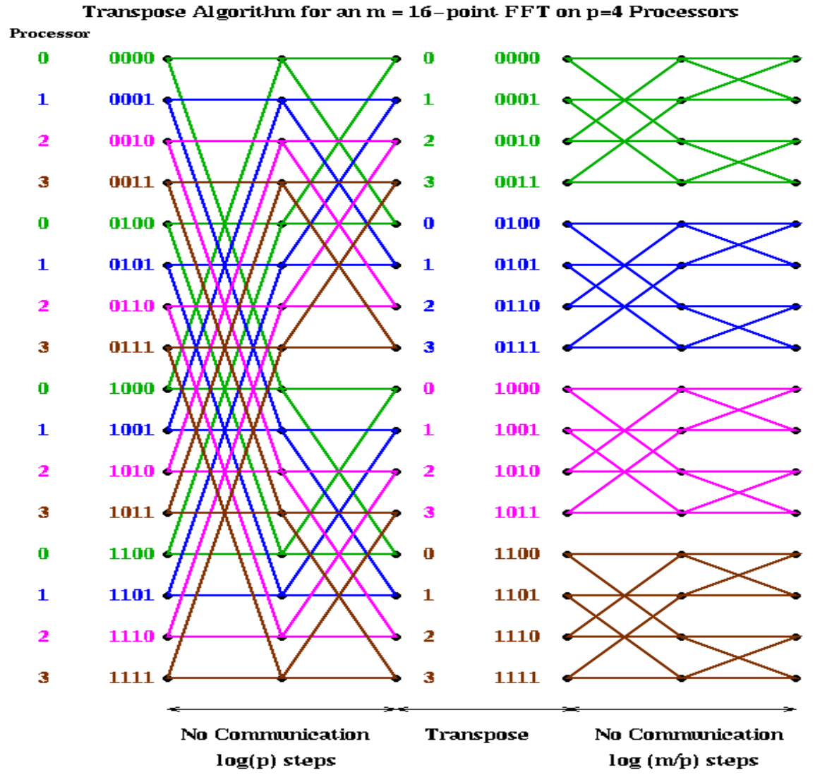
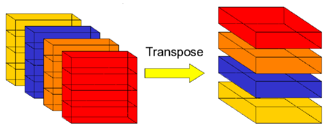
 There are cases in which neither of the above communication patterns is ideal. Instead, the first lg(P) steps can be performed with a cyclic data layout, so that there is no inter-processor communication required. Then, a single all-to-all communication step can be performed to achieve a blocked data layout. Then the final lg(m/P) steps require no inter-processor communication. The image below demonstrates this implementation. This communication pattern is called a “Corner-Turn” and resembles a transpose of a P × (m/P) distributed-memory matrix.
In a multi-dimensional problem, a similar set of problems arise. For example, suppose a 3-dimensional problem space where the data is decomposed among P processors by dividing along a single dimension, say Z. The “Butterfly” transforms along the two non-divided dimensions call all be performed without communication, since each processor owns entire slabs of the X × Y problem. A Corner-Turn exchange can be performed in order to obviate repeated communication phases during the Z-dimension FFT.
Invariants
Many fast O(n lg(n)) implementations of Fourier Transforms require changes to the data- layout; for example, may FFT implementations return data in bit-reversed-index order. Either the computations in the frequency domain must understand this ordering, or the program must pay the extra overheads of permuting the output data.
Examples
Note: example taken from Tim Mattson’s CS294 slides.
Given a complex-valued, periodic fuction of two variables:
g(x,y) = g(x+2π,y) = g(x,y+2π)
We wish to find a numerical solution for the function f (x, y) such that:
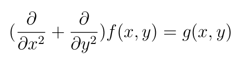
If we substitute the 2D Discrete Fourier Transforms for f and g:
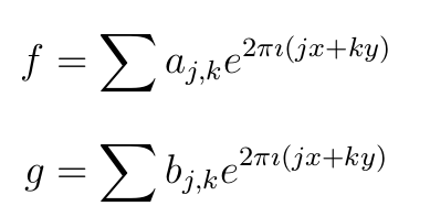
We obtain the equation:
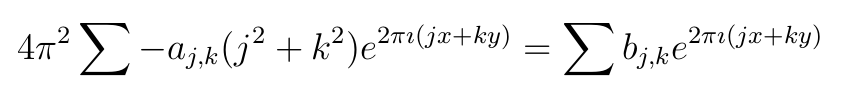
Having eliminated the partial derivatives, the solution, in terms of the Fourier coefficients, is now entirely algebraic:
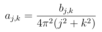
To obtain our numerical solution, we therefore need only to perform a 2-Dimensional Fourier Transform on the function g(x, y) to obtain the Fourier coefficients bj,k , scale the bj,k appropriately, and perform a 2-Dimensional Inverse Fourier Transform.
Known Uses
Related Patterns
Pipe-and-Filter, Linear Algebra, Structured Grids.
Author
Mark Murphy, citing Jim Demmel, Rajesh Nishtala, and Tim Mattson
The book “Chebyshev and Fourier Spectral Methods”, second edition, by John P. Boyd served as a primary reference for much of the background material.