Contents
Problem
A problem in 2, 3 or 4 dimensions, easily described with a structured grid which can be implemented as a n-dimensional array. Each update on the data is local in the physical space. How do you design an efficient solver which provides these updates and scales to many processors?
Context
In science and engineering it is often necessary to solve a problem represented by a grid of points and the value of a point in space is updated by a function of other nearby points. The value could, for example, represent the strength of an electric potential, the temperature of an oven or the color of a pixel in an image. Data is arranged in a regular multidimensional grid, usually in two or three dimensions. Computation proceeds as a sequence of grid update steps.
The location of nodes in the physical space directly maps to their location in data array (this is in contrast to the Unstructured Grid where the location of the element in the array cannot be directly inferred from the physical location).
The updates are logically concurrent, but in practice are implemented as a sequential sweep through the computational domain. Updates may be in place, overwriting the previous version, or use two versions of the grid. These codes have a high degree of parallelism, and data access patterns are regular and statically determinable.
The updates are usually done until the system reaches a particular error threshold. For example this is relevant to the case of partial differential equation solvers where the threshold is treated as the difference between successive iterations of the update algorithm. The solver iterates until the error threshold is reached.
Forces
The following forces create tensions which determine the architecture of the structured grid pattern:
-
Task granularity and parallelism: The problem needs to be broken down into tasks which may be processed in parallel. However, these tasks should not be so fine- grained that the resulting overhead of invoking these tasks reduces efficiency of parallelism. Tasks which are too simple for each processing element may result in high communication and initialization overheads and not enough processor utilization which will hinder scalability, while excessively complex tasks may result in unexploited parallelism.
-
Simple task partitioning and load balancing: The problem should be partitioned across processing elements in a simple efficient way. Each processing element is assigned a subproblem from the global domain, however the workload associated with each subproblem might not the equal. If this is the case, we need to perform load balancing in order to ensure equal distribution of work across all processing elements.
-
Performance and generality: The primary goal in structured grid problems is to solve the full problem as quickly as possible.However, some code transformations and changes to data layout/access which provide sequential performance gains may impede effective parallelization.
Solution
The first task of solving a problem with a structured grid pattern is the domain decomposition. To decompose the problem into tasks, the grid is sliced into contiguous chunks, and each processing element is assigned a chunk for work. The size of the chunk is determined by considering two factors:
-
the granularity of chunks needs to be small enough to exploit parallelism
-
the size of each chunk needs to be large enough to exploit computational resources of each processing element.
Thus, the ideal size of the chunks is determined by the specific parameters of the problem being solved and the number of available processing units. For more details see Geometric Decomposition pattern.
Stencils
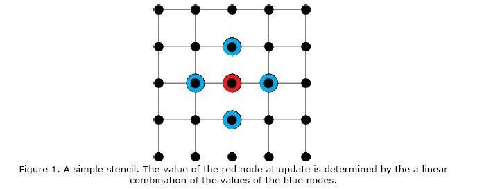
There are often one or few distinct dependencies for any given problem. The update rule is represented by a “stencil,” a linear combination of nearby nodes, named for its repetitious reproduction over the solution region. The values live in a finite geometric region, where the they are arranged in a regular fashion (as opposed to an unstructured grid, where dependencies, adjacencies, and locations of points can be highly irregular, see Unstructured Grid pattern).
Single-level regular N-dimensional grids
A simpler case of a structured grid pattern is solving problems mapped to 1, 2 or 3 dimensional grids. Each processor is assigned a chunk of the grid that is statically or dynamically determined by a partitioning algorithm. Each processor then computes the updates of the grid points in its chunk of data in each iteration.
“Ghost” nodes
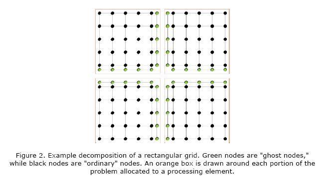
To deal with border grid points that require information located on other processors “ghost” nodes are usually used.
“Ghost” nodes contain all of the information necessary in order to update the subproblem at any particular processing element. They contain duplicate data in nodes present in adjacent chunks allocated to other processors. These updates are are synchronized across processors in order to hide latency in communication. “Ghost” nodes can be a single layer or multiple layers depending on the problem structure. Iteration for a single subproblem is referred to as a “local update,” reflecting the influence of the ghost points being felt only within the subproblem.
Double-buffering
A double-buffering-type approach may be used to perform the local updates, where two copies of the data are maintained–one for the data under construction and one for the data from the previous iteration. This allows for non-blocking concurrent access to the values needed to update the system. This is particularly useful in shared-memory systems where each processor may have access to an entire subproblem.
Advanced Solvers (Multi-Grid)
An optimization that can be made to the structured grid solver is to use multi-grids. Instead of partitioning the problem domain into fixed sized chunks, several copies of the grid are made at various chunk granularities. When a result from one node in the grid needs to be propagated to a different node a few chunks away, we move to a coarser grained grid thus making this update happen faster. This adds some computational complexity to the algorithm since we need to be able to map from one grid to the other, but it greatly speeds up convergence.
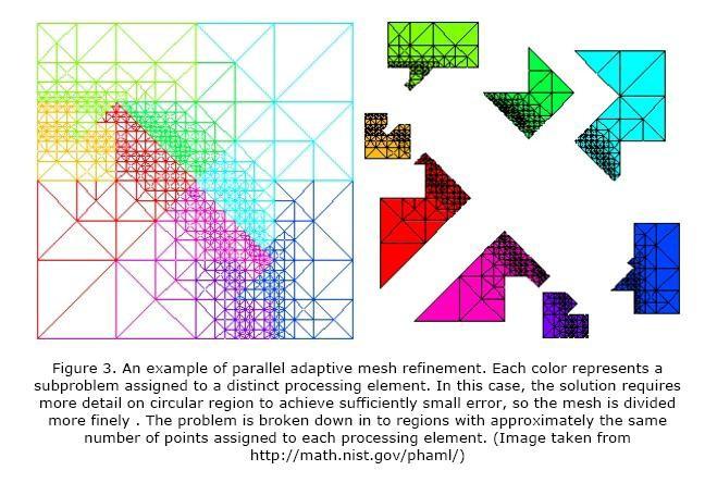
Adaptive Mesh Refinement
The structured grid problem may have both an error threshold and an underlying continuous space or region which the solution represents in discretized form. This solution may converge slowly or not at all depending on the spacing chosen for the discretization and the error tolerance. By using a discretization which is finer in certain regions, especially where the solution changes more rapidly in space or time, the convergence rate can be vastly improved. This approach is termed “adaptive mesh refinement”. After each update we check the solution and make a decision about whether to subdivide the region into smaller grid spacing.
In the parallel case, we partition the solution into contiguous chunks with ghost nodes at the edges, except now the partitioning of work may be less geometrically regular. This most likely will require a more intelligent task manager to ensure load balancing, as the division of work across processing elements may change as the discretization is refined. Task partitioning, however, is not an extremely difficult problem since the time required to perform a local update is ordinarily a simple function of the number of grid points enclosed. Interpolating between higher and lower resolution discretization can require significant overhead.
Invariant
-
There is no communication between processing elements on a given refinement level, except to update the ghost nodes on adjacent chunks.
-
Only one or a small number of prior iterations influences the value of a future iteration.
Examples
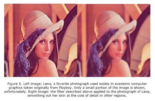
Example 1. Gaussian image blurring
To blur an image, , we set the value of a point equal to a weighted average of nearby points. In the continuous domain, this can be represented by a normal distribution in two dimensions, where u and v are image coordinates and sigma is a parameter controlling the extent of the blurring:
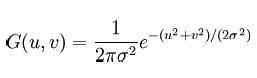
This equation is discretized into a stencil, represented as a matrix. The center value below is highlighted in bold, to indicate that the position of pixels is evaluated relative to that point. The new value for the “bold” pixel is given by the sum of the numbers below multiplied by the value of the pixel they represent.
0.00000067 0.00002292 0.00019117 0.00038771 0.00019117 0.00002292 0.00000067
0.00002292 0.00078633 0.00655965 0.01330373 0.00655965 0.00078633 0.00002292
0.00019117 0.00655965 0.05472157 0.11098164 0.05472157 0.00655965 0.00019117
0.00038771 0.01330373 0.110981640.225083520.11098164 0.01330373 0.00038771
0.00019117 0.00655965 0.05472157 0.11098164 0.05472157 0.00655965 0.00019117
0.00002292 0.00078633 0.00655965 0.01330373 0.00655965 0.00078633 0.00002292
0.00000067 0.00002292 0.00019117 0.00038771 0.00019117 0.00002292 0.00000067
Table 1. Gaussian blurring stencil for 3 pixel distance influence, with sigma set to 0.84. Values in each cell represent the integral of the distribution function over the extent of the pixel. (Table source: Wikipedia.)
In the example above, the image is a regular grid, partitioned across processing elements. Each processing element gets a submatrix of the image and performs updates to each pixel using the information from the neighboring pixels. We use a 49 point 2-dimensional stencil and the ghost zones are the three nodes out from the update point. In this case, we need the ghost nodes if we are using a distributed memory system since it will reduce the amount of computation needed for each iteration. If we have a shared memory machine, ghost nodes are not needed – each processor can access each pixel in the image concurrently, however care must be taken to avoid false sharing of cache lines (see the Shared Data (?) pattern).
Since this is a simple 2-dimensional grid and we perform one update iteration in solving this problem we do not need to use advanced methods such as multi-grid and adaptive mesh refinement.
Example 2. The Jacobi Scheme
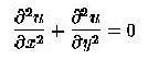
The Laplace equation is important in many fields of science such as electromagnetism and fluid dynamics. The equation describes the distribution of electric and fluid potentials in a medium. The Laplace equation can be solved efficiently using iterative methods over a structured grid.
The Laplace equation is as follows:
(1)
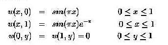
Where u = u(x, y) is an unknown scalar potential subjected to the following boundary conditions:
(2)
We discretize the equation numerically with centered difference and we obtain:
(3)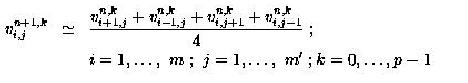
where n and n+1 denote the current and the next time step respectively while represents:
(4)![]()
The analytical solution for this boundary value problem can easily be verified to be:
(5)![]()
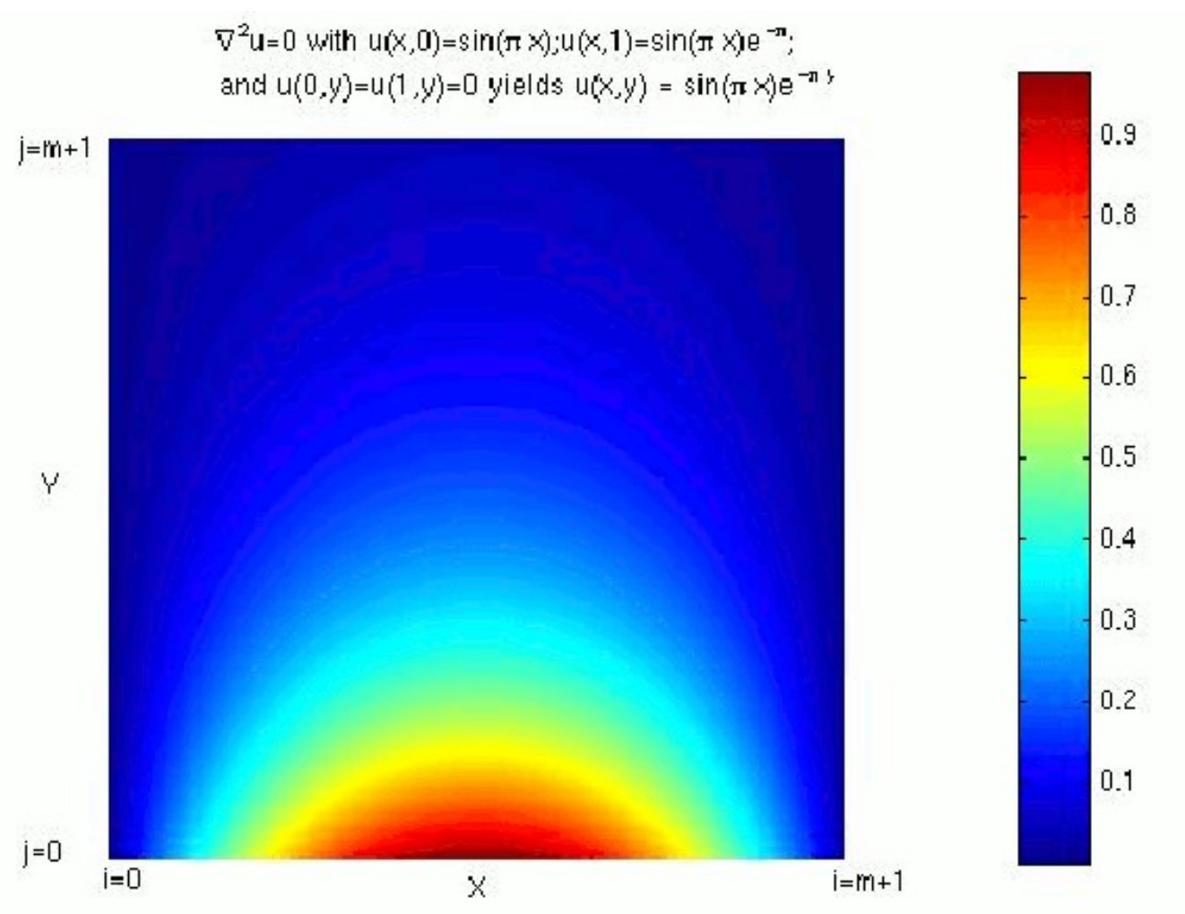
Figure 6: Contour Plot showing the analytical solution to the boundary value problem of finding the electric potential
The Jacobi Scheme is an iterative method that is used for solving such PDE’s as the Laplace equation. The simplest of the techniques is described as follows:
-
Make initial guess for u(i,j) at all interior points (i,j) for all i = 1:m and j=1:m
- Use centered difference equation (Eq3) to compute un+1i,j at all interior points(i,j)
-
Stop if the convergence threshold is reached, otherwise continue to the next step 4.
- uni,j = un+1i,j
- Go to Step 2.
To solve this problem in parallel, first we divide up the work among processors. Since the governing equation is two-dimensional we can use 1D or 2D decomposition. 1D decomposition assigns horizontal strips of the domain to each processor, while 2D decomposition assigns blocks.
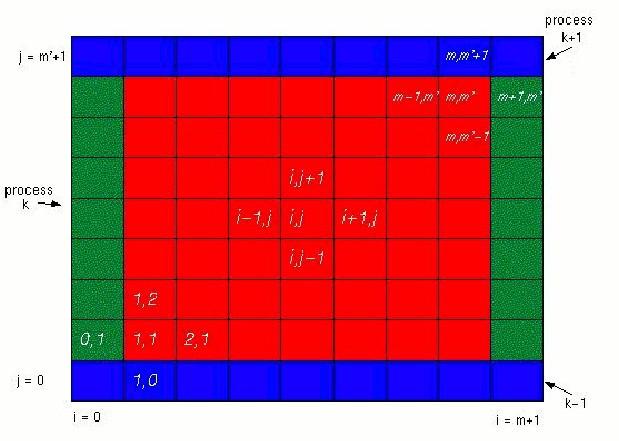
Figure 7: A sample grid allocation for one processor. The red is the inner nodes computed by 4-point stencils blue and green are “ghost” nodes.
In this case we have 4-point stencils and “ghost” nodes contain one level of nodes on the border of the processor’s grid chunk. The process iterates until the error threshold is reached.
The Jacobi iteration is the simplest way of solving this problem and it’s convergence rate is slow. More sophisticated methods can be used such as the Successive Over Relaxation (SOR) scheme, please see [11] for more details on how to parallelize SOR.
Example 3. The Finite Difference Method
Consider a simple problem: there is a rod of uniform material, it is insulated except at the ends.
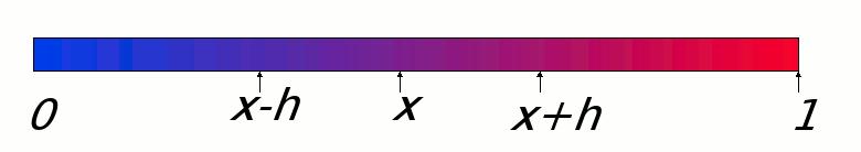
Let u(x,t) be the temperature at position x at time t. The heat travels from x-h to x+h at rate proportional to:
![]()
as h goes to 0, we get the heat equation:
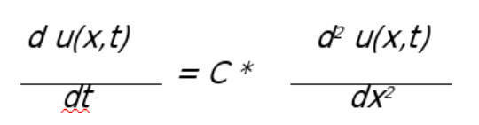
to solve this problem we discretize time and space using the forward Euler approach to approximate the time derivative with a difference:
to solve this problem we discretize time and space using the forward Euler approach to approximate the time derivative with a difference:
u(x,t+δ) – u(x,t))/δ= C [ (u(x-h,t)-u(x,t))/h – (u(x,t)- u(x+h,t))/h ] / h
= C[u(x-h,t) – 2*u(x,t) + u(x+h,t)]/h2
Solving foru(x,t+δ) we get:
u(x,t+δ) = u(x,t)+ C*δ/h2*(u(x-h,t) – 2*u(x,t) + u(x+h,t))
Letz=C*δ/h2, simplify:
u(x,t+δ) = z* u(x-h,t) + (1-2z)*u(x,t) + z*u(x+h,t)
Change variable x to j*h, t to i*δ, and u(x,t) to u[j,i], and thus we get:
u[j,i+1]=z*u[j1,i]+(12*z)*u[j,i]+z*u[j+1,i]
Now to solve this problem we use the finite difference method with u[j,i] as the temperature at time t, where t = i * δ(i = 0,1,2…) and position x = j * h(j = 0, 1, … N = 1/h). We set the initial conditions on u[j, 0] and boundary conditions on u[0, I] and u[N, I] according to the problem parameters. This results in a simple loop of iterations over j:
For j=0 to N
u[j,i+1]= z*u[j-1,i]+ (1-2*z)*u[j,i] + z*u[j+1,i] where z =C*δ/h2
where z=C*δ/h2
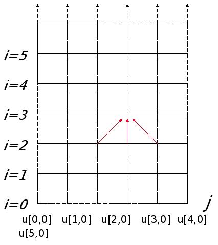
Figure 6: 1-dimensional Structured Grid used in solving the Head Equation with Finite Difference Method.
The value at every point in the grid is retrieved by a function of its three neighbors, this gives us a 3 point stencil. The grid can be partitioned across processing units in units of strips or blocks. The “ghost” nodes contain one extra level of the grid for each processor. The solver iterates till the system converges to a solution. Since the rod is uniform and the computation is fairly simple, advanced methods such as multi-grid and mesh refinement are not needed here.
Known Uses
The structured grid pattern is used nearly any place a partial differential equation is solved. Electromagnetic and electrostatic modeling for the design of electromagnetic equipment such as antennae, motors, circuitry, photonic devices, wave guides, and fiber optics are some examples of such problems. It is useful in oil finding via seismic inverse scattering, which is the eikonal partial differential equation. Structured grids are also seen in multimedia processing and structural mechanics applications. Interesting recent applications include sub-wavelength lithography simulation and biomolecule electrostatics calculations, especially for molecular dynamics.
Related Patterns
Structured grid is related to the following patterns:
1. Geometric Decomposition: this is the essence of the task manager described in the solution, used to intelligently subdivide the grid into chunks which are expected to have similar runtime.
2. Sparse Linear Algebra: when a node is a linear function of its neighbors, which is nearly always the case, a structured grid problem may be represented as the a large sparse matrix.
3. Unstructured grids: though interactions between data points are sparse in both cases, an unstructured grid may have a highly irregular spatial distribution and
adjacency of data points, and their interactions may be highly non-uniform.
4. N-body: the structured grid can be seen as the antithesis to the N-body problem, as the interactions between data points are extremely sparse.
References
1. Morton, K. W. and Mayers, D. F. 1995. Numerical Solution of Partial Differential Equations. Cambridge University Press.
2. Iserles, A. 1996 A First Course in the Numerical Analysis of Differential Equations.
Cambridge University Press.
3. MGNet Home Page. Craig C. Douglas. (Resource for domain decomposition and multigrid methods.) May 2008. http://www.mgnet.org/.
4. Structured Grids – A View From Berkeley. http://view.eecs.berkeley.edu/wiki/ Structured_Grids.
5. Timothy Mattson, Beverly Sanders, and Berna Massingill. 2004. Patterns for Parallel Programming (Software Patterns Series). Addison-Wesley Professional.
6. Tim Mattson. Mesh lecture. https://bspace.berkeley.edu/access/content/group/ 4d2145b3-4213-440f-801a-fce296ad9774/Slides/lecture6_meshes.pdf.
7. James D. Foley, Andries van Dam, Steven K. Feiner, John F. Hughes. 1995.
Computer Graphics: Principles and Practice in C (2nd Edition) (Systems
Programming Series). Addison-Wesley Professional.
8. Gaussian Blur – Wikipedia, the free encyclopedia. May 2008.
http://en.wikipedia.org/wiki/Gaussian_blur.
9. Finite Element Method – Wikipedia, the free encyclopedia. May 2008.
http://en.wikipedia.org/wiki/Finite_element_method.
10. Demmel, James. “CS267 Spring 2009 Lecture 7: Sources of Parallelism and Locality in Simulation” February 2009. _http://www.cs.berkeley.edu/~demmel/cs267_Spr09/
Lectures/lecture07_sources2jwd09.ppt
11. Boston University Scientific Computing and Visualization Group. “Example: Iterative Solvers”. http://scv.bu.edu/documentation/tutorials/MPI/alliance/apply/solvers/
Authors
Katya Gonina, Hovig Bayandorian
Shepherds
Erich Strohmaier