Problem
We can’t measure everything we need to know, and measurements are always noisy. How do we make use of the measurements we can perform to understand our data?
Context
Many problems in engineering and the sciences revolve around making measurements and inferring things about the forces which gave rise to the measurements. Measurements are always uncertain, and our understanding of the forces generating measurements is usually somewhat simplified, leading to errors between our idealized un- derstanding of a situation and the data we observe.
The most natural way to reason about this problem is through the use of probability theory. The measure- ments are modeled as random variables, and the forces which give rise to the measurements become probability distributions over these variables.
Additionally, our knowledge of a problem gives rise to structures relating different sets of measurements to different forces in our underlying problem. We should take advantage of our understanding of the problem to restrict the probability distributions to things which fit our models of the underlying problem and the measurement process.
Forces
1. Richer models with more degrees of freedom allow for modeling more complex phenomena, but also can lead to overfitting the data, leading to wrong conclusions
2. Usually, we don’t know exactly what model led to our data, so we have to guess. This leads to tension, since we need to choose a model that is as ”simple as possible, but not simpler”.
3. Sometimes we have to choose a simpler model because we understand it well and know how to apply it, but not because we’re sure our data was generated by that model (e.g., the well loved and but only sometimes justified Gaussian distribution.)
Invariants
1. Probability distributions must always sum to 1.
The solution to this problem is to capture the probability distributions as a graphical model. A graphical model formalizes the structure of the dependencies between random variables. It also drastically reduces the number of degrees of freedom in our probability distributions, making it possible for us to reason about the data we can collect and make inferences about the things we can’t measure directly.
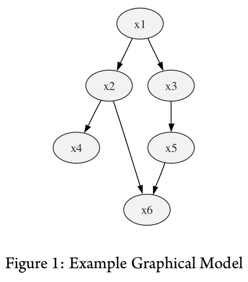
Figure 1: Example Graphical Model
For example, consider the graphical model shown in figure 1. The structure of the graph tells us which ran- dom variables are related to others. This is very important information that allows us to represent any probability distribution satisfying this model as follows:
p(x1, x2, x3, x4, x5, x6) = p(x1)p(x2|x1)p(x3|x1)p(x4|x2)p(x5|x3)p(x6|x2, x5)
Representing the distributions in this fashion makes reasoning about large networks of random variables prac- tical. There are three main tasks that we can accomplish once we have a graphical model:
1. Inference: Given a set of observed variables and probability distributions relating the variables, what are the probability distributions of the hidden variables?
2. Maximum a Posteriori Estimation: Given a set of observed variables, what is the most likely configuration of the hidden variables?
3. Parameter Estimation: Given a set of observed variables, what can we learn about the probability distribu- tions relating the variables?
When implementing computations using graphical models, one choice that needs to be made early is whether the computation is going to be performed exactly or approximately.
The canonical method for solving exact inference and estimation problems on graphical models is the Junction Tree Algorithm, which subsumes many special purpose algorithms developed for specific graphical models, such as the Viterbi algorithm for inference and the Baum-Welch algorithm for parameter estimation on Hidden Markov Models. The junction tree algorithm requires performing some graph transformations, including triangulation, on the graphical model in order to derive a junction tree. Because finding the optimal factorization is NP-hard, it is typical to attempt many randomized factorizations and then select the best (e.g., smallest maximal clique). This search can be rather trivially parallelized. The computations then center around passing messages regarding the probabilities of various quantities around this junction tree. Deriving these probabilities involves summing or maximizing local probability distributions.
Approximate inference algorithms can be applied when deterministic inference is not tractable. One approach involves propagating probability information around directly on the graphical model, which is not guaranteed to produce the correct result, but can work on some graphs. Other approaches involve dynamically limiting the prob- ability information which is passed around on the graph in order to avoid considering huge amounts of unlikely possibilities (ie, beam search.) Yet another approach is to sample from the joint distribution of random variables under consideration. The quality of the approximation is related to the number of random samples.
Examples
…
Known Uses
Speech and handwriting recognition technology is based on the Hidden Markov Model framework, which is a tree- structured graphical model. A subset of the nodes are observed as a sequence of acoustic or visual evidence, and the task involves inferring the underlying state sequences corresponding to linguistic structure. The forward-backward algorithm (SUM-PRODUCT) is used for exact inference of posterior probabilities during model training (with the EM algorithm). The Viterbi algorithm is used for MAP estimation of the most likely hypothesis.
Junction Tree Algorithms have been used in some speech recognition systems for factorizing a Dynamic Bayesian Network, a generalization of the HMM.
Monte Carlo methods are usually applied with graphical models in computational physics, in which the struc- ture is typically a highly-coupled grid.
Authors
Bryan Catanzaro and Arlo Faria