Pipeline

Problem

Suppose that the overall computation involves performing a calculation on many sets of data, where the calculation can be viewed in terms of data flowing through a sequence of stages. How can the potential concurrency be exploited?

Context

An assembly line is a good analogy for this pattern. Suppose we want to manufacture a number of cars. The manufacturing process can be broken down into a sequence of operations each of which adds some component, say the engine or the windshield, to the car. An assembly line (pipeline) assigns a component to each worker. As each car moves down the assembly line, each worker installs the same component over and over on a succession of cars. After the pipeline is full (and until it starts to empty) the workers can all be busy simultaneously, all performing their operations on the cars that are currently at their stations.

Examples of pipelines are found at many levels of granularity in computer systems, including the CPU hardware itself.

• Instruction pipeline in modern CPUs. The stages (fetch instruction, decode, execute, memory stage, write back, etc.) are done in a pipelined fashion; while one instruction is being decoded, its predecessor is being executed and its successor is being fetched.
• Vector processing (loop­level pipelining). Specialized hardware in some supercomputers allows operations on vectors to be performed in a pipelined fashion. Typically, a compiler is expected to recognize that a loop such as

for (i=0; i<N; i++) { a[i] = b[i] + c[i]; } in assembly:
    li vlr, 64 # vector length is 64
    lv v1, r1 # load vector b from memory lv v2,
    r2 # load vector c from memory addv.d
    v3, v1, v2 # add vector a = b + c sv v3, r3 # store vector a to memory

can be vectorized in a way that the special hardware can exploit. After a short startup, one a[i] value will be generated each clock cycle.

• Algorithm ­level pipelining. Many algorithms can be formulated as recurrence relations and implemented using a pipeline or its higher‐ dimensional generalization, a systolic array. Such implementations often exploit specialized hardware for performance reasons.
• Signal processing. Passing a stream of real‐time sensor data through a sequence of filters can be modeled as a pipeline, with each filter corresponding to a stage in the pipeline.
• Graphics. Processing a sequence of images by applying the same sequence of operations to each image can be modeled as a pipeline, with each operation corresponding to a pipeline stage. Some stages may be implemented by specialized hardware.
• Shell programs in UNIX. For example, the shell command

cat file | grep “word” | wc –l

creates a three‐stage pipeline, with one process for each command (cat, grep, and wc)

These examples and the assembly‐line analogy have several aspects in common. All involve applying a sequence of operations (in the assembly line case it is installing the engine, installing the windshield, etc.) to each element in a sequence of data elements (in the assembly line, the cars). Although there may be ordering constraints on the operations on a single data element (for example, it might be necessary to install the engine before installing the hood), it is possible to perform different operations on different data elements simultaneously (for example, one can install the engine on one car while installing the hood on another.)

The possibility of simultaneously performing different operations on different data elements is the potential concurrency this pattern exploits. Each task consists of repeatedly applying an operation to a data element (analogous to an assembly‐line worker installing a component), and the dependencies among tasks are ordering constraints enforcing the order in which operations must be performed on each data element (analogous to installing the engine before the hood).

Forces

Universal forces

• Deep pipeline or short pipeline (Throughput or latency). There is a design decision when using a Pipeline pattern. If the throughput is important the depth of the pipeline should be deep, if the latency is important the depth of the pipeline should be short. However, if the depth of the pipeline gets shorter, the amount of parallelism decreases.
• In many situations where the Pipeline pattern is used, the performance measure of interest is the throughput, the number of data items per time unit that can be processed after the pipeline is already full. For example, if the output of the pipeline is a sequence of rendered images to be viewed as an animation, then the pipeline must have sufficient throughput (number of items processed per time unit) to generate the images at the required frame rate.
• In another situation, the input might be generated from real‐ time sampling of sensor data. In this case, there might be constraints on both the throughput (the pipeline should be able to handle all the data as it comes in without backing up the input queue and possibly losing data) and the latency (the amount of time between the generation of an input and the completion of processing of that input). In this case, it might be desirable to minimize latency subject to a constraint that the throughput is sufficient to handle the incoming data.

Implementation forces

• Multiprocessors on one node or several nodes on a cluster. You might end up using one node that has several cores or using more nodes on a cluster. If you use several nodes, the communication cost is normally expensive than using several cores on one node, so the amount of work expected before communication on each compute node should be larger.
• Special purpose hardware or general purpose hardware. If you use special purpose hardware to exploit parallelism, there might be certain restriction in the future when modifying the pipeline. However, if you use a general purpose hardware the peak performance you might achieve could not be as competitive when using a special purpose hardware such as vector machines.

Solution

The key idea of this pattern is captured by the assembly‐line analogy, namely that the potential concurrency can be exploited by assigning each operation (stage of the pipeline) to a different worker and having them work simultaneously, with the data elements passing from one worker to the next as operations are completed. In parallel‐programming terms, the idea is to assign each task (stage of the pipeline) to a UE and provide a mechanism whereby each stage of the pipeline can send data elements to the next stage. This strategy is probably the most straightforward way to deal with this type of ordering constraints. It allows the application to take advantage of special‐purpose hardware by appropriate mapping of pipeline stages to PEs and provides a reasonable mechanism for handling errors, described later. It also is likely to yield a modular design that can later be extended or modified.

 

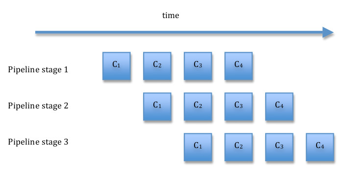
Before going further, it may help to illustrate how the pipeline is supposed to operate. Let C_i represent a multistep computation on data element i. C_i(j) is the jth step of the computation. The idea is to map computation steps to pipeline stages so that each stage of the pipeline computes one step. Initially, the first stage of the pipeline performs C₁(1). After that completes, the second stage of the pipeline receives the first data item and computes C₁(2) while the first stage computes the first step of the second item, C₁(1). Next, the third stage computes C₁(3), while the second stage computes C₂(2) and the first stage C₃(1). The figure above illustrates how this works for a pipeline consisting of four stages. Notice that concurrency is initially limited and some resources remain idle until all the stages are occupied with useful work. This is referred to as filling the pipeline. At the end of the computation (draining the pipeline), again there is limited concurrency and idle resources as the final item works its way through the pipeline. We want the time spent filling or draining the pipeline to be small compared to the total time of the computation. This will be the case if the number of stages is small compared to the number of items to be processed. Notice also that overall throughput/efficiency is maximized if the time taken to process a data element is roughly the same for each stage.

This idea can be extended to include situations more general than a completely linear pipeline. For example, the figure below illustrates two pipelines, each with four stages. In the second pipeline, the third stage consists of two operations that can be performed concurrently.

Linear Pipeline

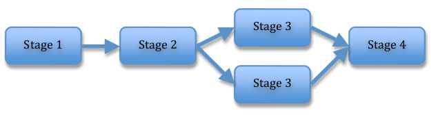Nonlinear Pipeline

Define the stages of the pipeline. Normally each pipeline stage will correspond to one task. The figure below shows the basic structure of each stage.

initialize
while (more data)
{
    receive data element from previous stage 
    perform operation on data element
    send data element to next stage
}
finalize

If the number of data elements to be processed is known in advance, then each stage can count the number of elements and terminate when these have been processed. Alternatively, a sentinel indicating termination may be sent through the pipeline.

It is worthwhile to consider at this point some factors that affect performance.

• The amount of concurrency in a full pipeline is limited by the number of stages. Thus, a larger number of stages allows more concurrency. However, the data sequence must be transferred between the stages, introducing overhead to the calculation. Thus, we need to organize the computation into stages such that the work done by a stage is large compared to the communication overhead. What is “large enough” is highly dependent on the particular architecture. Specialized hardware (such as vector processors) allows very fine‐grained parallelism.
• The pattern works better if the operations performed by the various stages of the pipeline are all about equally computationally intensive. If the stages in the pipeline vary widely in computational effort, the slowest stage creates a bottleneck for the aggregate throughput.
• The pattern works better if the time required to fill and drain the pipeline is small compared to the overall running time. This time is influenced by the number of stages (more stages means more fill/drain time).

Therefore, it is worthwhile to consider whether the original decomposition into tasks should be revisited at this point, possibly combining lightly‐loaded adjacent pipeline stages into a single stage, or decomposing a heavily‐loaded stage into multiple stages.

It may also be worthwhile to parallelize a heavily‐loaded stage using one of the other Parallel Algorithm Strategy patterns. For example, if the pipeline is processing a sequence of images, it is often the case that each stage can be parallelized using the Task Parallelism pattern.

Structure the computation. We also need a way to structure the overall computation. One possibility is to use the SPMD pattern and use each UE’s ID to select an option in a case or switch statement, with each case corresponding to a stage of the pipeline.

To increase modularity, object‐oriented frameworks can be developed that allow stages to be represented by objects or procedures that can easily be “plugged in” to the pipeline. Such frameworks are not difficult to construct using standard OOP techniques, and several are available as commercial or freely available products.

Represent the dataflow among pipeline elements. How dataflow between pipeline elements is represented depend on the target platform.

In a message‐passing environment, the most natural approach is to assign on process to each operation (stage of the pipeline) and implement each connection between successive stages of the pipeline as a sequence of messages between the corresponding processes. Because the stages are hardly ever perfectly synchronized, and the amount of work carried out at different stages almost always varies, this flow of data between pipeline stages must usually be both buffered and ordered. Most message‐passing environments (e.g., MPI) make this easy to do. If the cost of sending individual messages is high, it may be worthwhile to consider sending multiple data elements in each message; this reduces total communication cost at the expense of increasing the time needed to fill the pipeline.

If a message‐passing programming environment is not a good fit with the target platform, the stages of the pipeline can be connected explicitly with buffered channels. Such a buffered channel can be implemented as a queue shared between the sending and receiving tasks, using the Shared Queue pattern.

If the individual stages are themselves implemented as parallel programs, then more sophisticated approaches may be called for, especially if some sort of data redistribution needs to be performed between the stages. This might be the case if, for example, the data needs to be partitioned along a different dimension or partitioned into a different number of subsets in the same dimension. For example,  an application might include one stage in which each data element is partitioned into three subsets and another stage in which it is partitioned into four subsets. Simple ways to handle such situations are to aggregate and disaggregate data elements between stages. One approach would be to have only one task in each stage communicate with tasks in other stages; this task would then be responsible for interacting with the other tasks in its stage to distribute input data elements and collect output data elements. Another approach would be to introduce additional pipeline stages to perform aggregation/disaggregation operations. Either of these approaches, however, involves a fair amount of communication. It may be preferable to have the earlier stage “know” about the needs of its successor and communicate with each task receiving part of its data directly rather than aggregating the data at one stage and then disaggregating at the next. This approach improves performance at the cost of reduced simplicity, modularity, and flexibility.

Less traditionally, networked file systems have been used for communication between stages in a pipeline running in a workstation cluster. The data is written to a file by one stage and read from the file by its successor. Network file systems are usually mature and fairly well optimized, and they provide for the visibility of the file at all PEs as well as mechanisms for concurrency control. Higher‐level abstractions such as tuple spaces and blackboards implemented over networked file systems can also be used. File‐system‐based solutions are appropriate in large‐ grained application in which the time needed to process the data at each stage is large compared with the time to access the file system.

Handling errors. For some applications, it might necessary to gracefully handle error conditions. One solution is to create a separate task to handle errors. Each stage of the regular pipeline sends to this task any data elements it cannot process along with error information and then continues with the next item in the pipeline. The error task deals with the faulty data elements appropriately.

Processor allocation and task scheduling. The simplest approach is to allocate one PE to each stage of the pipeline. This gives good load balance if the PEs are similar and the amount of work needed to process a data element is roughly the same for each stage. If the stages have different requirements (for example, one is meant to be run on special‐purpose hardware), this should be taken into consideration in assigning stages to PEs.

If there are fewer PEs than pipeline stages, then multiple stages must be assigned to the same PE, preferably in a way that improves or at least does not much reduce overall performance. Stages that do not share many resources can be allocated to the same PE; for example, a stage that writes to a disk and a stage that involves primarily CPU computation might be good candidates to share a PE. If the amount of work to process a data element varies among stages, stages involving less work may be allocated to the same PE, thereby possibly improving load balance. Assigning adjacent stages to the same PE can reduce communication costs. It might also be worthwhile to consider combining adjacent stages of the pipeline into a single stage.

If there are more PEs than pipeline stages, it is worthwhile to consider parallelizing one or more of the pipeline stages using an appropriate Algorithm Structure pattern, as discussed previously, and allocating more than one PE to the parallelized stage(s). This is particularly effective if the parallelized stage was previously a bottleneck (taking more time than the other stages and thereby dragging down overall performance).

Another way to make use of more PEs than pipeline stages, if there are no temporal constraints among the data items themselves (that is, it doesn’t matter if, say, data item 3 is computed before data item 2), is to run multiple independent pattern. This will improve the latency, however, since it still takes the same amount of time for a data element to traverse the pipeline.

Examples

Fourier-­transform computations. A type of calculation widely used in signal processing involves performing the following computations repeatedly on different sets of data.

1. Perform a discrete Fourier transform (DFT) on a set of data.
2. Manipulate the result of the transform elementwise.
3. Perform an inverse DFT on the result of the manipulation.

Examples of such calculations include convolution, correlation, and filter operations.

A calculation of this form can easily be performed by a three stage pipeline.

• The first stage of the pipeline performs the initial Fourier transform; it repeatedly obtains one set of input data, performs the transform, and passes the result to the second stage of the pipeline.
• The second stage of the pipeline performs the desired elementwise manipulation; it repeatedly obtains a partial result (of applying the initial Fourier transform to an input set of data) from the first stage of the pipeline, performs its manipulation, and passes the result to the third stage of the pipeline. This stage can often itself be parallelized using one of the other Algorithm Structure patterns.
• The third stage of the pipeline performs the final inverse Fourier transform; it repeatedly obtains a partial result (of applying the initial Fourier transform and then the elementwise manipulation to an input set of data) from the second stage of the pipeline, performs the inverse Fourier transform, and outputs the result.

Each stage of the pipeline processes one set of data at a time. However, except during the initial filling of the pipeline, all stages of the pipeline can operate concurrently, while the (N‐1)‐th set of data, and the third stage is processing the (N‐ 2)‐the set of the data.

Let’s see an example of a low pass filter. In order to avoid implementation specifics of a DFT and an inverse DFT, this example uses MATLAB. The DFT function in MATLAB is fft2, and the inverse DFT function in MATLAB is ifft2. The three stages explained are the following.

(1) Read the image file and do a DFT.

>> lena = imread(‘lenagray.bmp’);
>> imshow(lena);
>> lenadft = fft2(double(lena)); % do a dft
>> imshow(real(fftshift(lenadft))); % display the dft

(2) Crop a circle out.

>> [M,N] = size(lenadft);
>> u = 0:(M-1);
>> v = 0:(N-1);
>> idx = find(u>M/2);
>> u(idx) = u(idx) - M;
>> idy = find(v>N/2);
>> v(idy) = v(idy) - N;
>> [V,U] = meshgrid(v,u);
>> D = sqrt(U.^2+V.^2);
>> P = 20; H = double(D<=P); % make mask of size P
>> lenalowpass = lenadft .* H;
>> imshow(H);
>> imshow(real(fftshift(lenalowpass)));

(3) Do an inverse DFT.

>> lenanew = real(ifft2(double(lenalowpass)));
>> imshow(lenanew, [ ]);

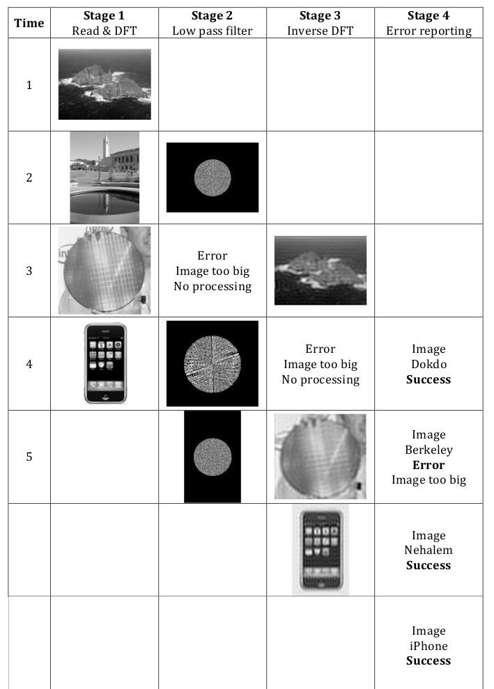
Let’s see how the actual pipeline works. Due to the limited resources, let’s assume that the machine can only process an image smaller than 512 pixels x 512 pixels. If an image larger than this size comes in, the pipeline should report an error, though it should not affect other images in the pipeline. In this case we need another stage for error handling. In this diagram, the time flows from top to the bottom.

We have four images, which are Dokdo, Berkeley, Nehalem, and iPhone. The Berkeley image’s height is 540 pixels so it should trigger an error.

Known uses

Many applications in signal and image processing are implemented as pipelines. The OPUS [SR98] system is a pipeline framework developed by the Space Telescope Science Institute originally to process telemetry data from the Hubble Space Telescope and later employed in other applications. OPUS uses a blackboard architecture built on top of a network file system for interstage communication and includes monitoring tools and support for error handling.

Airborne surveillance radars use space‐time adaptive processing (STAP) algorithms, which have been implemented as a parallel pipeline [CLW+ 00]. Each stage is itself a parallel algorithm, and the pipeline requires data redistribution between some of the stages.

Fx [GOS94], a parallelizing Fortran compiler based on HPF [HPF97], has been used to develop several example applications [DGO+94, SSOG93] that combine data parallelism (similar to the form of parallelism captured in the Geometric Decomposition pattern) and pipelining. For example, one application performs 2D fourier transforms on a sequence of images via a two‐stage pipeline (one stage for the row transforms and one stage for the column transforms), with each stage being itself parallelized using data parallelism. The SIGPLAN paper [SSOG93] is especially interesting in that it presents performance figure comparing this approach with a straight data‐parallelism approach.

[J92] presents some finer‐grained applications of pipelining, including inserting a sequence of elements into a 2‐3 tree and pipelined mergesort.

Related patterns

Pipe­ and ­filter pattern. This pattern is very similar to the Pipe­and­Filter pattern; the key difference is that this pattern explicitly discusses concurrency.

Task Parallelism pattern. For applications in which there are no temporal dependencies between the data inputs, an alternative to this pattern is a design based on multiple sequential pipelines executing in parallel and using the Task Parallelism pattern.

Discrete Event pattern. The Pipeline pattern is similar to the Discrete Event pattern in that both patterns apply to problems where it is natural to decompose the computation into a collection of semi‐independent tasks. The difference is that the Discrete Event pattern is irregular and asynchronous where the Pipeline pattern is regular and synchronous: In the Pipeline pattern, the semi‐independent tasks represent the stages of the pipeline, the structure of the pipeline is static, and the interaction between successive stages is regular and loosely synchronous. In the Discrete Event pattern, however, the tasks can interact in very irregular and asynchronous ways, and there is no requirement for a static structure.

References

[SR98] Daryl A. Swade and James F. Rose. OPUS: A flexible pipeline data‐processing environment. In Proceedings of the AIAA/USU Conference on Small Satellites. September 1998.

[CLW+00] A. Choudhary, W. Liao, D. Weiner, P. Varshney, R. Linderman, and R. Brown. Design, implementation, and evaluation of parallel pipelined STAP on parallel computers. IEEE Transactions on Aerospace and Electronic Systems, 36(2):528‐548, April 2000.

[GOS94] Thomas Gross, David R. O’Hallaron, and Jaspal Subhlok. Task parallelism in a High Performance Fortran framework. IEEE Parallel & Distributed Technology, 2(3):16‐26, 1994.

[HPF97] High Performance Fortran Forum: High Performance Fortran Language specification, version 2.0

[DGO+94] P. Dinda, T. Gross, D. O’Hallaron, E. Segall, J. Stichnoth, J. Subhlock, J. Webb, and B. Yang. The CMU task parallel program suite. Technical Report CMU‐ CS‐94‐131, School of Computer Science, Carnegie Mellon University, March 1994.

[SSOG93] Jaspal Subhlok, James M. Stichnoth, David R. O’Hallaron, and Thomas Gross. Exploiting task and data parallelism on a multicomputers. In Proceedings of the Fourth ACM SIGPLAN Symposium on Principles and Practice of Parallel Programming. ACM Press, May 1993.

[J92] J.JaJa. An Introduction to Parallel Algorithms. Addison‐Wesley, 1992.

Author

Modified by Yunsup Lee, Ver 1.0 (March 11, 2009), based on the pattern “Pipeline Pattern” described in section 4.8 of PPP, by Tim Mattson et.al.