SIMD

Problem

How do you exploit concurrency defined as parallel updates to data without specifying in detail how that concurrent execution is implemented?

Context

Programmers tend to think of a program’s execution as a sequence of instructions. The program’s source code may include many branches with multiple pathways through the code, but only one path at a time is active. When concurrent execution is needed, however, this way of thinking about the program’s execution is usually inadequate: In many parallel algorithms, different pathways through a program may be active at the same time, or there may be multiple UEs3 executing the same code at the same time but more or less independently. This parallel mindset has proved very difficult for programmers to master.

It would be valuable if we could define a high-level abstraction that allows program- mers to think in terms of a single thread of control, with the concurrency being hidden inside lower-level primitives. Defining a high-level abstraction for the general case has proved difficult if not impossible. However, there is a subset of problems for which it is easier: those where the concurrency is defined in terms of largely independent up- dates to the elements of the key data structures in the problem. For such problems, the data-parallel model, in which the program appears to have a single thread of control, but operations on these key data structures are implicitly concurrent, seems reasonable.

This is a particularly attractive model for some hardware platforms, particularly those involving groups of processing elements that can readily be made to operate in a SIMD (Single Instruction, Multiple Data) style. Several programming environments for such platforms are based on this model; they typically provide predefined datatypes suitable for these key data structures and ways of operating on them in parallel.

Forces

All the program structure patterns in PLPP share a common set of forces, described in some detail in [MSM04] and summarized here, with discussion of how they apply to the SIMD pattern in particular.

• Clarity of abstraction. Is the parallel algorithm clearly apparent from the source code?

Code that allows the reader to see the details of the algorithm with little mental effort is always important for writing correct code, but is particularly essential for parallel programs.

It is particularly important if the target hardware platform is one that may be difficult to program at a low level (as is the case with some hardware platforms involving special-purpose processors).

• Scalability. How many processors can the parallel program effectively utilize?

Scalability of a program is restricted by three factors: the amount of concurrency
available in the algorithm, the fraction of the runtime spent doing inherently
serial work, and the parallel overhead of the algorithm.

The importance of scalability relative to other goals may depend in part on the target hardware platform (i.e., what constraints exist on the maximum number of processing elements). However, it is always important to be sure the amount of exploitable concurrency is large enough, the serial fraction of the code small enough, and the overhead small enough to allow the algorithm to make good use of whatever processing elements are available. Notice that for target hardware platforms where the data-parallel operations are executed on a coprocessor (such as a GPU), overhead can include the cost of moving or copying data between host memory and the coprocessor.

• Efficiency. How close does the program come to fully utilizing the resources of the parallel computer?

Quantitatively, efficiency is typically measured by comparing the time taken by the best sequential algorithm to the time taken by the parallel algorithm multi- plied by the number of processing elements.

• Maintainability. Is the program easy to debug, verify, and modify?

Programs that are difficult to understand are usually also difficult to get running in the first place, and to modify throughout their lifetimes. Parallel programs are notoriously difficult to debug, especially if programmers cannot understand them without reasoning about multiple independent threads of control interacting in different ways.

• Environmental affinity. Is the program well aligned with the programming environment and hardware of choice?

Whenever feasible, program designs should be portable to as many platforms as possible, but in any case it should be possible to implement them efficiently on likely target platforms.

• Sequential equivalence. Where appropriate, does a program produce equiva- lent results when run with many UEs as with one? If not equivalent, is the relationship between them clear?

It is highly desirable that the results of an execution of a parallel program be the same regardless of the number of processing elements used. This is not always possible, because changes in the order of floating-point operations can produce small (or not so small, if the algorithm is not well-conditioned) changes in results. However, it is highly desirable, since it allows us to reason about correctness and do most testing on a single-process version of the program.

Solution

The SIMD pattern is based in general on the data-parallel model described in the Con- text section, and in particular on the SIMD style. The pattern is based on two key ideas: (1) organizing the data relevant to a problem into regular iterative data struc- tures such as arrays, which we will call parallel data structures, and (2) defining the computation in terms of a sequence of parallel updates to these parallel data structures. Often in applying these two ideas one must also introduce parallel data structures to hold intermediate results.

Notice that the meaning of a data-parallel program can be understood in terms of a sequence of instructions, in much the same way as a sequential program. The concur- rency is hidden inside the updates to the elements of the parallel data structures. This is valuable to a programmer trying to understand a new program and also in debugging.

Applying this pattern is often best done using the strategy of incremental parallelism described in the PLPP Loop Parallelism and Reengineering for Parallelism patterns. Consider a sequential program that we wish to execute on parallel hardware, such as a GPU or a multi-core processor. An effective and practical approach to incrementally transforming the code into a parallel program is as follows.

• Identify exploitable concurrency. Find the bottlenecks in the program and the data structures central to the computation. In cases where this pattern is effective, these will often appear as computations organized as loops over all elements of an array. Notice that you may need to restructure the problem to recast it into this form.
• Refactor to eliminate obstacles to parallelism. Eliminate loop-carried depen- dencies, and express each computation as a simple loop over all elements of an array, where all the iterations are independent.
• Revise to use data-parallel operations. Recast the loop body as a data-parallel operation on the array using the data-parallel operations provided by the target programming environment. (If the environment provides both a foreach construct and whole-array operations, consider making this transformation in two stages: First replace the loop with a foreach and verify that the result is correct. Then replace the foreach with a whole-array operation or operations.)
• Allocate elements to threads (if needed). Allocate elements of the array to threads. In some environments, this task is taken care of by the compiler/runtime system combination. In others, it is explicitly managed by the programmer, who needs to be aware of the resources of the specific hardware.
• Tune for performance. Build the program and evaluate the effectiveness of the solution so far. Is there enough work done on each element to justify the overhead? In a multi-core environment, the overhead comes from creating and managing the threads. There should be enough work per thread to make this worthwhile. If a coprocessor is being used, the overhead tends to be dominated by the cost of transferring data between the host and coprocessor memory. In addition, coprocessors may not have caches, so the number of memory accesses should be minimized.

The following short examples are typical of the kinds of transformations that can be helpful in applying this pattern. These examples, like the longer code examples later in the pattern, are in Fortran 95. A short summary of its relevant features appears in the section “Example Programming Environment (Fortran 95)” below.

• Replacing loops with foreach (forall) constructs and then array operations is fairly straightforward.

For example, suppose you start with arrays x, y, and z with indices ranging from 1 to N and a calculation of the form

do i = 1, N
  z(i) = a * x(i) + y(i)

Since the iterations of the loop are independent, this can be readily transformed to use a forall as follows

forall (i = 1 : N)
  z(i) = a * x(i) + y(i) 
end forall

and further transformed to use array operations as follows

z = a * x + y;

• The PLPP Algorithm Structure pattern Task Parallelism discusses several techniques for eliminating loop-carried dependencies, most involving replacing a sin- gle variable with one copy per UE. These same techniques can be applied here, replacing single variables with arrays.

For example, suppose you start with a calculation of the form

do i = 1, numSteps 
  x = x + f(i)

This can be transformed by introducing an array y to hold intermediate results which are later combined, giving

forall (i = 1 : numSteps) 
  y = f(i)
end forall
x = sum(y) ! library function, returns sum of elements of array

Performance Considerations

In order for this pattern to be effective, the following two conditions must be met.

• The arrays, or the work per element, must be large enough to compensate for overheads inherent in managing the parallel execution.
• A large enough fraction of the computation must fit this pattern to keep the se- rial fraction low; otherwise overall scalability will be limited, as described by Amdahl’s law.

The pattern also must be appropriate for the hardware target. A common use of this pattern is for general-purpose programming of a GPU. In this case, the GPU serves as a coprocessor. This adds a number of extra costs:

• The data must be marshaled into a buffer for movement to the coprocessor.
• The data must be moved from the CPU address space into the coprocessor ad- dress space.
• The computations must be managed to satisfy any synchronization constraints between the coprocessor and the CPU.
• The results must be moved from the coprocessor address space back to the CPU address space.

The time required for these steps must be small compared to the runtime on the copro- cessors if this pattern is to be effective.

Programming Environments

This pattern works best when the target programming environment makes it easy to express parallel data structures and operations. Such environments usually provide the following high-level constructs.

• Element-wise basic arithmetic operations.
• Common collective operations such as scatter, gather, reduction, and prefix scan.
• A foreach command to handle more general element-wise updates.

Examples of such environments include the following.

• Fortran 95 [MR96, IBM]. Many of the array operations in Fortran 90 were de- signed to allow compilers to exploit vector-processing or other parallel hardware if available; Fortran 95 added a forall construct similar to the foreach described above.
• High Performance Fortran (HPF) [HPF97]. HPF is a set of extensions to For- tran 90 for data-parallel computing. It includes some of the additions of For- tran 95 (e.g., forall), compiler directives for indicating how arrays should be distributed among UEs, and additional library functions.
• The PeakStream Platform [Pea]. This platform provides C/C++ library classes and functions to define and operate on parallel arrays.
• Microsoft’s Accelerator [Acc]. This system, aimed at facilitating general- purpose use of GPUs, provides C# library classes to define and operate on paral- lel arrays.

Example Programming Environment (Fortran 95)

In this section we briefly describe the features of Fortran 95 that make it a data-parallel programming environment. This is the environment we chose for the code examples in this pattern, largely because there are free compilers readily available for common platforms, so the code can be compiled and its correctness verified without requiring special software or hardware.

• Whole-array operations. As an example of operations on arrays, consider the following code fragment to compute the product of a scalar value a and an array x, add it to an array y, and assign the result to array z. Indices for each array range from 1 to N, where N is an integer defined elsewhere.

real a
real x(1:N), y(1:N), z(1:N)
z = a * x + y

• A forall construct similar to the foreach mentioned earlier. A Fortran 95 forall consists of a range of index values and a “loop body” of statements to be executed for each index in the range. Assignment statements in the loop body work as parallel assignments, with all right-hand sides evaluated before values are assigned to any left-hand sides. We could rewrite the preceding example using this construct as follows:

real a
real x(1:N), y(1:N), z(1:N)
forall (i = 1 : N)
  z(i) = a * x(i) + y(i) 
end forall

This construct also includes an optional mask specifying that the loop body is to be executed only for indices that match a particular criterion. For example, the following code changes all negative elements of array x to zero.

real x(1:N)
forall (i = 1 : N, x(i) < 0) 
  x(i) = 0.0
end forall

Examples

As examples of this pattern in action, we will consider in some detail the following, and then briefly describe other examples and known uses.

• Computing π using numerical integration. (This example is used in several pat- terns of PLPP.)
• Simplified modeling of heat diffusion in a one-dimensional pipe, as an example of a mesh computation. (This example is also used in several patterns of PLPP.)
• The Black-Scholes method for option pricing, a widely used example of Monte Carlo methods.
• The so-called scan problem, a generalized version of computing partial sums of an array.

Numerical Integration

Consider the problem of estimating the value of π using the following equation.

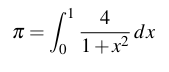
We can use the midpoint rule to numerically approximate the integral. The idea is to approximate the area under a curve using a series of rectangles, as shown in Fig. 1.

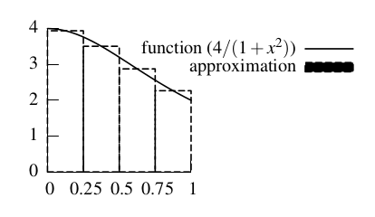
Figure 1: Approximating the area under a curve with a series of rectangles. Notice that the width of each rectangle is the width of the whole area divided by the number of rectangles, and the height of each rectangle is the value of the function at the x coordinate in the middle of the rectangle.

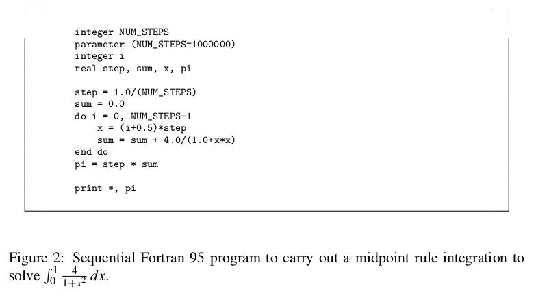
A program to carry this calculation out on a single processor is shown in Fig. 2. To keep the code simple, we hard-code the number of rectangles (steps). The variable sum is initialized to zero and the step size is computed as the range in x (equal to 1.0 in this case) divided by the number of steps. The area of each rectangle is the width (the step size) times the height (the value of the integrand at the center of the interval), as shown in Fig. 1. Since the width is a constant, we pull it out of the summation and multiply the sum of the rectangle heights by the step size, step, to get our estimate of the definite integral.

Since we are beginning with sequential code, we can work through the steps described previously for a strategy based on making changes incrementally, as follows.

Identify exploitable concurrency. The only source of exploitable concurrency is the iterations of the loop, and they are almost independent and therefore a good fit for the simplest of the PLPP Algorithm Structure patterns, Task Parallelism.

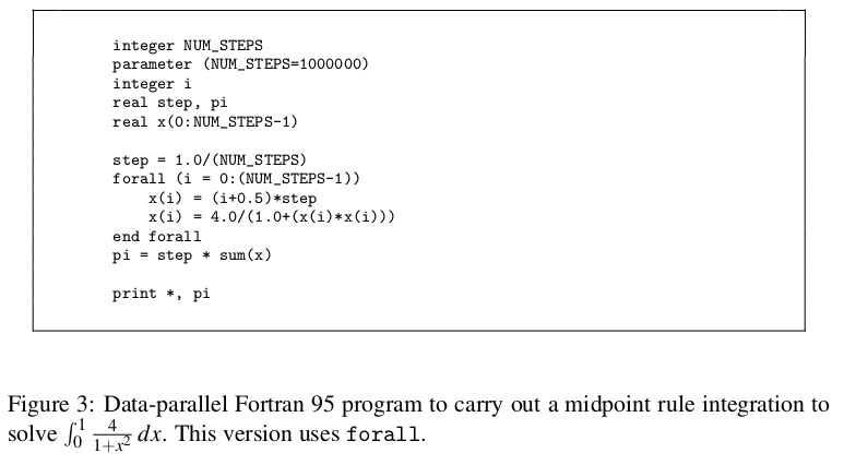
Refactor to eliminate obstacles to parallelism. As discussed in Task Parallelism, the single loop-carried dependency is the summing of intermediate values into sum, which we can eliminate by having each thread of control compute its own partial sum and combining them at the end. We can do this in a way that fits with the data-parallel model by simply replacing temporary variable x with an array to hold the intermediate values that will be summed. We can then compute the intermediate results by per- forming operations on this array, ending with a reduction operation to compute their sum.

Revise to use data-parallel operations. Following the strategy of making changes incrementally, we could start by making the changes just described and replacing the do loop with a forall, as shown in Fig. 3.

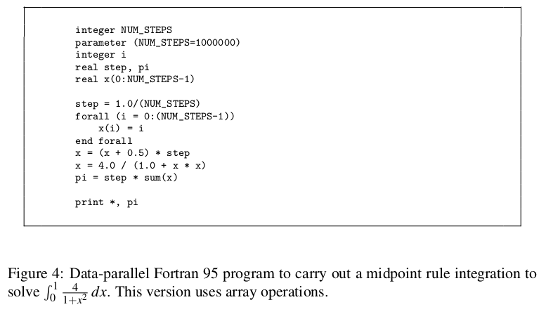
Further revise to use more-data-parallel operations. We can then make the pro- gram more purely data-parallel by replacing each line of the body of the forall with an element-wise operation on the array x, as shown in Fig. 4. (We do still have to use a forall to give each element of the array a value based on its index. Some program- ming environments might provide a library function that would do this, however.)

Concluding remarks. Two of the PLPP program structure patterns, SPMD and Loop Parallelism, also discuss this example. Both use the same strategy presented here (com- puting partial sums and combining them); only the way in which this strategy is turned into code is different.

Mesh Computation

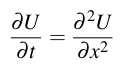
The problem is to model one-dimensional heat diffusion (i.e., diffusion of heat along an infinitely narrow pipe). Initially the whole pipe is at a stable and fixed temperature. At time 0, we set both ends to different temperatures, which will remain fixed throughout the computation. We then calculate how temperatures change in the rest of the pipe over time. (What we expect is that the temperatures will converge to a smooth gradient from one end of the pipe to the other.) Mathematically, the problem is to solve a one- dimensional differential equation representing heat diffusion:

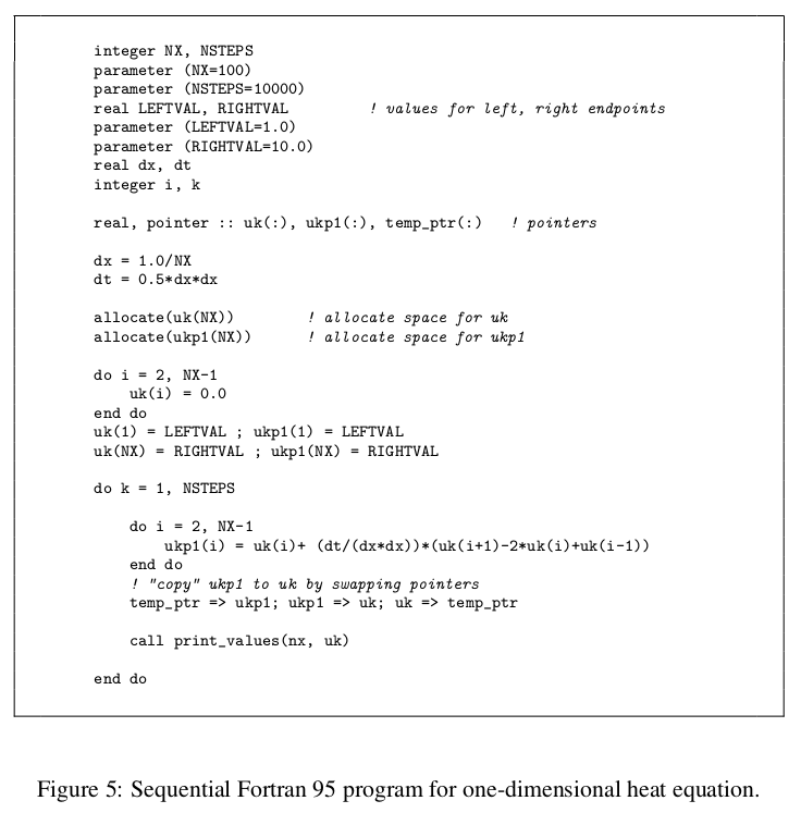
The approach used is to discretize the problem space (representing U by a one- dimensional array and computing values for a sequence of discrete time steps). We will output values for each time step as they are computed, so we need only save val- ues for U for two time steps; we will call these arrays uk (U at the timestep k) and ukp1 (U at timestep k + 1). At each time step, we then need to compute for each point in array ukp1 the following:

ukp1(i)=uk(i)+ (dt/(dx*dx))*(uk(i+1)-2*uk(i)+uk(i-1))

Variables dt and dx represent the intervals between discrete time steps and between discrete points respectively. A program to carry this calculation out on a single proces- sor is shown in Fig. 5. (Code for print_values is straightforward and not shown.) Notice that it employs a bit of cleverness to avoid copying values from ukp1 to uk at every time step: It defines pointers to the two arrays and simply swaps pointers, achieving the same result without the additional cost of copying the whole array.

Since we are beginning with sequential code, we can work through the steps de- scribed previously for a strategy based on making changes incrementally, as follows.

Identify exploitable concurrency. The overall calculation in this problem is a good fit for the PLPP Algorithm Structure pattern Geometric Decomposition, because the heart of the computation is repeated updates of a large data structure, namely ukp1.

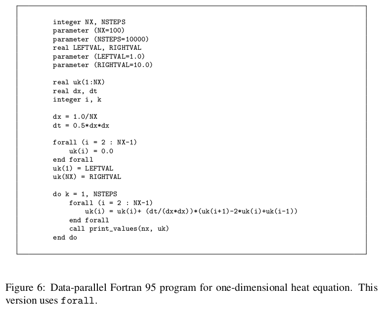
Revise to use data-parallel operations. Expressing the same calculation using data parallelism is actually simpler, however, given the semantics of the forall construct (as described in the section “Example Programming Environment (Fortran 95)” ear- lier); We can maintain a single copy of the array representing U and update all ele- ments in parallel, thus:

forall (i = 2 : NX-1)
  uk(i) = uk(i)+ (dt/(dx*dx))*(uk(i+1)-2*uk(i)+uk(i-1)) 
end forall

Fig. 6 shows the complete program.

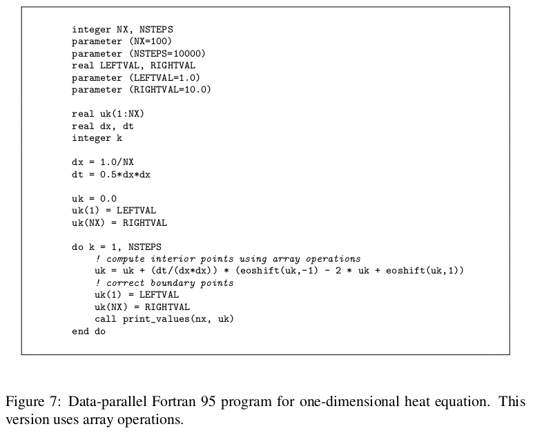
Further revise to use more-data-parallel operations. Alternatively, we could ex- press the required calculation in terms of operations on arrays, though it is slightly less straightforward to do so: Calculation of U for each point requires old values for the point itself and its left and right neighbors. Left and right neighbors are represented in the sequential code by array elements with indices i-1 and i+1. But element i-1 is just element i of the array formed by shifting all elements of uk to the right by one, and similarly for element i+1 and an array formed by shifting uk left. Fortran 95 has such a function, namely eoshift: eoshift(a,n) returns an array obtained by shifting a by n positions (left for positive n, right for negative n) and padding with zeros. We can use it to do the required calculation thus:

uk = uk + (dt/(dx*dx)) * (eoshift(uk,-1) - 2 * uk + eoshift(uk,1))

provided we then correct the wrongly-computed values for the first and last element (which are supposed to remain constant). Fig. 7 shows the complete program.

Concluding remarks. This example is discussed in some detail in text of Geometric Decomposition (in [MSM04]), and implementations using MPI and OpenMP are shown.

Black-Scholes Option Pricing

As an example of a calculation from a different domain area, namely finance, consider the Black-Scholes model for option pricing [BS73]. As commonly defined, an option is an agreement between a buyer and a seller, in which the buyer is granted a right (but not an obligation), secured by the seller, to carry out some operation (exercise the option) at some time in the future. The predetermined price is called the strike price, and the future date is called the expiration date. A call option grants the buyer the right to buy the underlying asset at the strike price; a put option grants the buyer the right to sell the underlying asset at the strike price. There are several types of options, mostly depending on when the option can be exercised; European options can be exercised only on the expiration date, while American-style options are more flexible. For a call option, the profit made is the difference between the price of the asset at the exercise date and the strike price, minus the option price. For a put option, the profit made is the difference between the strike price and the price of the asset at the exercise date, minus the option price. How much one would be willing to pay for the option therefore depends on many factors, including:

• Asset price at expiration date.
• Strike price.
• Time to expiration date. (Longer times imply more uncertainty.)
• Riskless rate of return, i.e., annual interest rate of bonds or other investments considered to be risk-free. P dollars invested at this rate will be worth P·e^rT dollars T years from now; equivalently, one gets P dollars T years from now by investing P·e^−rT dollars now.

The model gives a partial different equation for the evolution of an option price under certain assumptions. For European options, there is a closed-form solution to this PDE:

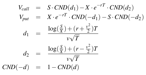
where

• V_call is the price for an option call
• V_put is the price for an option put
• CND(d) is the Cumulative Normal Distribution function
• S is the current option price
• X is the strike price
• T is the time to expiration
• r is the continuously compounded risk-free interest rate
• v is the implied volatility for the underlying asset

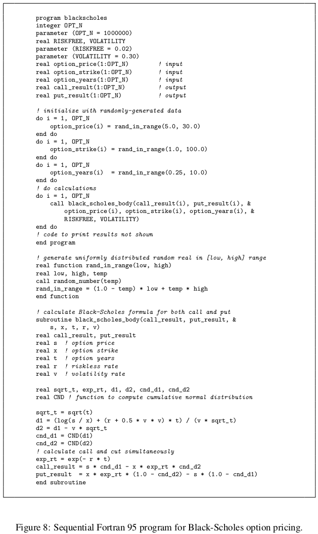
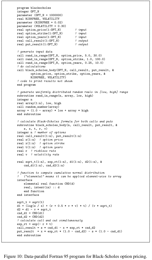
Fig. 8 shows code, based on similar code provided as one of the CUDA SDK exam- ples [NVI], that uses these equations to calculate V_call and V_put for a set of randomly- generated values of S, X , and T. To keep the code simpler, r, v, and the number of samples are hard-coded.

Since we are beginning with sequential code, we can work through the steps described previously for a strategy based on making changes incrementally, as follows.

Identify exploitable concurrency. There are four obvious sources of exploitable concurrency, corresponding to the four loops in the main program. For each loop, if its iterations are independent, or nearly so, then they can be executed concurrently, as described in simplest of the PLPP Algorithm Structure patterns, Task Parallelism.

Refactor to eliminate obstacles to parallelism. To find out whether the iterations are independent, we need to look at subprograms rand_in_range (for the first three loops) and black_scholes_body (for the fourth loop). We will assume that local variables for subprograms are allocated in a way that does not introduce dependencies between loop iterations (a reasonable assumption for Fortran 95 and probably for most target environments).

Looking first at rand_in_range, we observe that it in turn makes calls to random_number. This is a library function, and unless we can be sure it gives correct results even if multiple copies are invoked concurrently, we must regard its use as a loop-carried dependency, and this might mean that this loop would need to stay sequential. Fortunately, however, in addition to generating a single value, the library function is capable of generating multiple values into an array, and with a little refactoring of the sequential code we can make use of this feature to eliminate the first three loops, for example replacing

do i = 1, OPT_N
    option_price(i) = rand_in_range(5.0, 30.0) 
end do

with

call rand_in_range(OPT_N, option_price, 5.0, 30.0)

(This does not by any means guarantee that the library function will do anything con- currently, but it does allow us to express the computation in a way that is readily seen to be correct and easily mapped onto a library function for generating random values in parallel, if one exists in the target programming environment.)

 

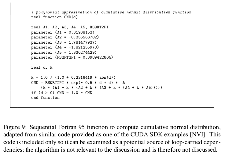
Looking next at black_scholes_body, we notice that it in turn makes calls to CND, but this function by inspection is safe for concurrent execution, since it uses only read-only constants and local variables. (Code for CND is given in Fig. 9.) So we should be able to replace this loop with a forall. Because of restrictions on what can be in the body of a forall construct, however, we cannot do this directly, but must refactor so that we pass whole arrays into black_scholes_body and perform the loop (to be replaced by a forall) inside the subroutine. The revised black_scholes_body will have the form

subroutine black_scholes_body(n, call_result, put_result, & s, x, t, r, v)
integer n ! number of options
real call_result(1:n), put_result(1:n), s(1:n), x(1:n), t(1:n) real r, v
real sqrt_t, exp_rt, d1, d2, cnd_d1, cnd_d2, CND 
integer i
do i = 1, n
    sqrt_t = sqrt(t(i))
    ! remaining lines similarly transformed
end do
end subroutine

When we do this, however, we introduce loop-carried dependencies for the interme- diate results (e.g., sqrt_t). These are readily addressed with the technique described earlier: Replace each variable used for an intermediate result with an array that can be operated on as a parallel data structure. So, for example, we could replace the declara- tion of sqrt_t with an array declaration

real sqrt_t(1:n)

and rewrite the first line of the loop thus

sqrt_t(i) = sqrt(t(i))

Revise to use data-parallel operations. At this point we can replace the loop in black_scholes_body with a forall. Following the strategy of making changes incrementally, at this point it would probably be wise to build the program and confirm that it produces correct output.

Further revise to use more-data-parallel operations. Finally, we can transform the forall construct into a sequence of whole-array operations; for example, the first line can be replaced with

sqrt_t = sqrt(t)

The complete program is shown in Fig. 10.

Scan

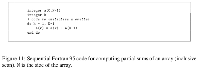
A simple but frequently useful operation is computing all partial sums of an array of numbers, sometimes called sum-prefix or all-prefix-sums. This operation can be generalized to a so-called scan operation (to use the terminology of APL [Ive62]). This operation requires a sequence a0, a1, . . . , an−1 and a binary operator ◦ with an identity element. Output is a new sequence with element i defined as

a0 ◦ a1 ◦ · · · ◦ ai

This is a so-called inclusive scan; if the sum does not include the element itself, it is called an exclusive scan. (It is clearly straightforward to convert between the two types of scans: inclusive to exclusive by shifting right one position, padding with the identity element, and exclusive to inclusive by shifting left one position and inserting as the last element the sum of the last element of the inclusive scan and the first element of the

original sequence.) Fig. 11 shows code for a naive sequential algorithm for an inclusive scan using addition.

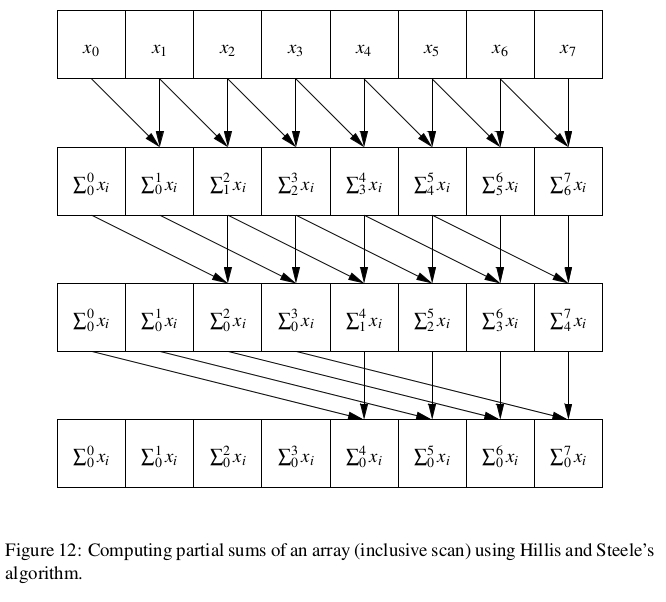
Although we are starting with sequential code, a strategy of incremental parallelism will not help here. Instead, what is needed is a rethinking of the problem. Hillis and Steele [HS86] point out that while this appears to be an inherently sequential operation with execution proportional to the length of the array, clever use of data parallelism can reduce the execution time from O(n) to O(log n), given enough processors to assign a processor to each element. A more work-efficient version of the algorithm was later proposed by Blelloch [Ble90]. The examples in [HS86] were part of the inspiration for one of the more interesting of the PLPP Algorithm Structure patterns, Recursive Data, which captures the overall strategy used both for Hillis and Steele’s parallel algorithm and for Blelloch’s modified version. In the rest of this section we discuss these two algorithms.

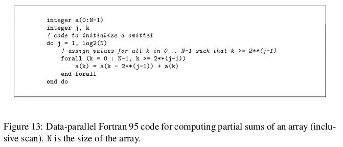
Hillis/Steele algorithm. The overall idea is to make log2 n passes through the array, where n is its size, first adding to each element k the (k − 1)-th element, then the (k − 2)-th element, then the (k − 4)-th element, and so forth, as illustrated in Fig. 12. Fig. 13 shows code for this algorithm. Notice that the body of the forall construct is executed only for indices that match the mask; in iteration j of the outer loop, the body of the forall will be executed only for those k for which k ≥ 2 j−1. Recall also that statements in the body of a forall operate as a parallel assignment; in this case, replacing the forall with a sequential loop would give a different and incorrect result.

However, although this algorithm is clever, and faster than the simple sequential version if there are enough processors, it achieves this result at a cost of more total work — O(n log n) operations total, as opposed to the O(n) operations required for the sequential algorithm. If there are significantly more array elements than processors, the data-parallel algorithm of Fig. 13 might even be slower than its sequential counterpart. Addressing this problem requires additional rethinking.

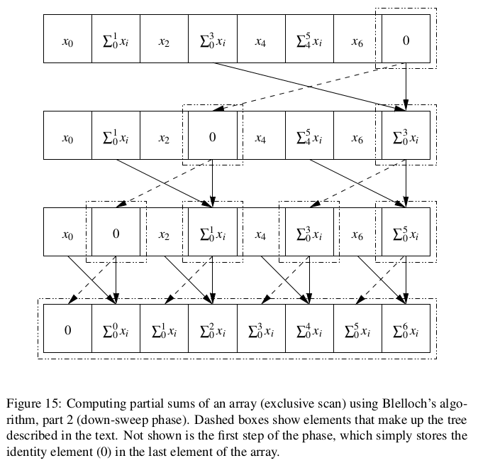
Blelloch algorithm. The idea of this more work-efficient algorithm is as follows: Conceptually build a binary tree based on the array, with leaf nodes corresponding to elements, and non-leaf nodes that combine successive nodes at the next lower level.

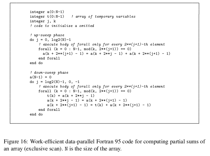
 (So for an array with 8 elements, the root node of the tree represents elements 0–7, the nodes one level down represent elements 0–3 and 4–7, and so forth.) Divide the computation into two phases, an up-sweep that moves up the tree computing partial sums, as illustrated in Fig. 14, and a down-sweep that uses these results to compute the desired prefix sums for all array elements, as illustrated in Fig. 15. Notice that this algorithm computes an exclusive scan rather than an inclusive one. Fig. 16 shows

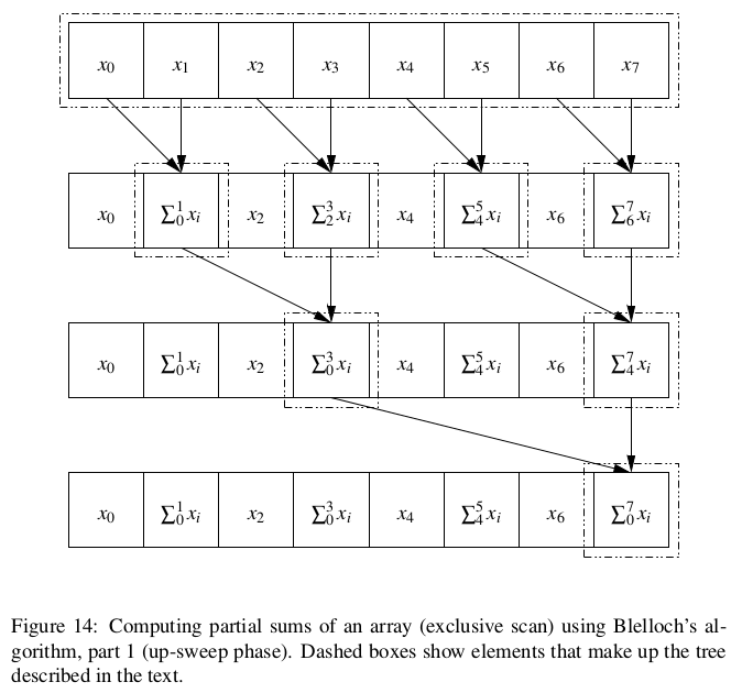
code for this algorithm. Notice that again we use a mask in the forall, this time to specify that in iteration j of the outer loop, the body of the forall will be executed only for those k for which (k mod 2^j+1) = 0 (i.e., every 2^j+1-th element). Recall also that statements in the body of a forall function as a parallel assignment; in this case, replacing the forall with a sequential loop would give a different and incorrect result.

Concluding remarks. It is worth remarking that neither of these algorithms would probably be used if the only goal were to compute partial sums of an array: The total amount of work even for a fairly large array is too small to justify the added complexity

and overhead, and this kind of calculation is common enough that the target program- ming environment might provide a library function for it. However, both algorithms are interesting in their own right, as illustrations that data parallelism is more broadly applicable than one might at first think. Further, either algorithm might be practical in the right setting — for example, if it were part of a larger calculation with enough total work to justify the overhead of managing data parallelism.

Known Uses

• Programs using one of the programming environments described earlier. Examples using Accelerator can be found in [TPO06]; examples using the PeakStream Platform can be found at the company’s Web site [Pea].
• Examples used in the PLPP Recursive Data pattern:
  • Finding, for each node in a forest of trees, the root of the tree to which it belongs, in time proportional to the logarithm of the height of the forest, as discussed in [J9´2].
  • Finding partial sums in a linked list, as discussed in [HS86].
• Other data-parallel algorithms from [HS86].

Related Patterns

The SIMD pattern joins and complements the other Supporting Structures patterns de- scribing program structure (SPMD, Loop Parallelism, and so forth). As described in [MSM04], which of these patterns to use for a particular application usually de- pends on a combination of target programming environment and the overall strategy for exploiting concurrency (i.e., which Algorithm Structure patterns are being used). Just as SPMD is a good fit for MPI and Loop Parallelism is a good fit for OpenMP, SIMD is a good fit if the target programming environment provides the features de- scribed in the Solution section of this pattern. An additional pattern at this level will probably be needed in order to properly address stream-processing programming en- vironments; these environments target similar hardware, but express calculations in terms of a kernel (sequence of instructions) operating in parallel on elements of a data structure (stream) rather than in terms of a single sequence of operations, each of which operates concurrently on elements of a data structure.

With regard to overall strategy, the Algorithm Structure patterns that map best to SIMD are Task Parallelism, Geometric Decomposition, and Recursive Data, since all have a kind of regularity that lends itself to being expressed in terms of operations on parallel data structures. The other Algorithm Structure patterns (Divide and Conquer, Pipeline, and Event-Based Coordination) do not map as well to SIMD.

Acknowledgments

We gratefully acknowledge the help of our shepherd for this paper. Danny Dig.

References

[Acc] Microsoft Accelerator. http://research.microsoft.com/research/ downloads/Details/25e1bea3-142e-%4694-bde5-f0d44f9d8709/ Details.aspx?CategoryID.

[Ble90] Guy E. Blelloch. Prefix sums and their applications. In John H. Reif, editor,
Synthesis of Parallel Algorithms. Morgan Kaufmann, 1990. [Bro] http://graphics.stanford.edu/projects/brookgpu/.
[BS73] Fischer Black and Myron Scholes. The pricing of options and corporate liabilities. Journal of Political Economy, 81(3):637–654, 1973.

[Fly72] M. J. Flynn. Some computer organizations and their effectiveness. IEEE Transactions on Computers, C-21(9), 1972.

[Hil85] W. Daniel Hillis. The Connection Machine. MIT Press, 1985.

[HPF97] High Performance Fortran Forum: High Performance Fortran Language specification, version 2.0. http://dacnet.rice.edu/Depts/CRPC/ HPFF, 1997.

[HS86] W. Daniel Hillis and Guy L. Steele, Jr. Data parallel algorithms. Commu- nications of the ACM, 29(12):1170–1183, 1986.

[IBM] IBM Corporation. XL Fortran for AIX 8.1 language reference. http://www.ncsa.uiuc.edu/UserInfo/Resources/Hardware/ IBMp690/IBM/usr/sh%are/man/info/en_US/xlf/html/lr.HTM.

[Ive62] Kenneth E. Iverson. A Programming Language. Wiley, 1962.
[J9´2] J. Ja´Ja´. An Introduction to Parallel Algorithms. Addison-Wesley, 1992. [MMS99] Berna L. Massingill, Timothy G. Mattson, and Beverly A. Sanders. Pat-
terns for parallel application programs. In Proceedings of the Sixth Pattern Languages of Programs Workshop (PLoP 1999), August 1999.

[MMS00] Berna L. Massingill, Timothy G. Mattson, and Beverly A. Sanders. Patterns for finding concurrency for parallel application programs. In Proceedings of the Seventh Pattern Languages of Programs Workshop (PLoP 2000), Au- gust 2000.

[MMS01] Berna L. Massingill, Timothy G. Mattson, and Beverly A. Sanders. More patterns for parallel application programs. In Proceedings of the Eighth Pattern Languages of Programs Workshop (PLoP 2001), September 2001.

[MMS02] Berna L. Massingill, Timothy G. Mattson, and Beverly A. Sanders. Some algorithm structure and support patterns for parallel application programs. In Proceedings of the Ninth Pattern Languages of Programs Workshop (PLoP 2002), September 2002.

[MMS03] Berna L. Massingill, Timothy G. Mattson, and Beverly A. Sanders. Ad- ditional patterns for parallel application programs. In Proceedings of the Tenth Pattern Languages of Programs Workshop (PLoP 2003), September 2003.

[MMS05] Berna L. Massingill, Timothy G. Mattson, and Beverly A. Sanders. Reengi- neering for parallelism: An entry point into PLPP (pattern language for par- allel programming) for legacy applications. In Proceedings of the Twelfth Pattern Languages of Programs Workshop (PLoP 2005), September 2005.

[MMS07] Berna L. Massingill, Timothy G. Mattson, and Beverly A. Sanders. Reengi- neering for parallelism: An entry point into PLPP (pattern language for par- allel programming) for legacy applications. Concurrency and Computation: Practice and Experience, 19(4):503–529, 2007.

[MR96] Michael Metcalf and John K. Reid. Fortran 90/95 Explained. Oxford Uni- versity Press, 1996.

[MSM04] Timothy G. Mattson, Beverly A. Sanders, and Berna L. Massingill. Patterns for Parallel Programming. Addison-Wesley, 2004. See also our Web site at http://www.cise.ufl.edu/research/ParallelPatterns.

[NVI] NVIDIA CUDA (Compute Unified Device Architecture). http:// developer.nvidia.com/object/cuda.html.

[Pea] The PeakStream platform. http://www.peakstreaminc.com/. [Rap] The RapidMind platform. http://www.rapidmind.net/.

[TPO06] David Tarditi, Sidd Puri, and Jose Oglesby. Accelerator: Using data par- allelism to program GPUs for general-purpose uses. In Proceedings of the 12th International Conference on Architectural Support for Programming Languages and Operating Systems. ACM Press, 2006.

Authors

Berna L. Massingill

Timothy Mattson

Beverly A. Sanders

A Review of PLPP

This section provides a brief overview of our pattern language (PLPP) as described in [MSM04], for the convenience of readers unfamiliar with the language.

The pattern language is organized into four design spaces, corresponding to the four phases of the underlying methodology and described in the subsequent sections. Pro- grammers normally start at the top (in Finding Concurrency) and work down through the other design spaces in order until a detailed design for a parallel program is obtained.

A.1 The Finding Concurrency Design Space

This design space is concerned with structuring the problem to expose exploitable con- currency. The designer working at this level focuses on high-level algorithmic issues and reasons about the problem to expose potential concurrency. Patterns in this space include the following.

• Decomposition patterns, used to decompose the problem into pieces that can execute concurrently:
  • Task Decomposition: How can a problem be decomposed into tasks that can execute concurrently?
  • Data Decomposition: How can a problem’s data be decomposed into units that can be operated on relatively independently?
• Dependency-analysis patterns, used to help group the tasks and analyze the de- pendencies among them:
  • Group Tasks: How can the tasks that make up a problem be grouped to simplify the job of managing dependencies?
  • Order Tasks: Given a way of decomposing a problem into tasks and a way of collecting these tasks into logically related groups, how must these groups of tasks be ordered to satisfy constraints among tasks?
  • Data Sharing: Given a data and task decomposition for a problem, how is data shared among the tasks?
• Design Evaluation: Is the decomposition and dependency analysis so far good enough to move on to the Algorithm Structure design space, or should the design be revisited?

A.2 The Algorithm Structure Design Space

This design space is concerned with structuring the algorithm to take advantage of potential concurrency. That is, the designer working at this level reasons about how to use the concurrency exposed in working with the Finding Concurrency patterns. The Algorithm Structure patterns describe overall strategies for exploiting concurrency. Patterns in this space include the following.

• Patterns for applications where the focus is on organization by task:
  • Task Parallelism: How can an algorithm be organized around a collection of tasks that can execute concurrently?
  • Divide and Conquer: Suppose the problem is formulated using the sequen- tial divide and conquer strategy. How can the potential concurrency be exploited?
• Patterns for applications where the focus is on organization by data decomposi- tion:
  • Geometric Decomposition: How can an algorithm be organized around a data structure that has been decomposed into concurrently updatable “chunks”?
  • Recursive Data: Suppose the problem involves an operation on a recursive data structure (such as a list, tree, or graph) that appears to require sequential processing. How can operations on these data structures be performed in parallel?
• Patterns for applications where the focus is on organization by flow of data:
  • Pipeline: Suppose that the overall computation involves performing a cal- culation on many sets of data, where the calculation can be viewed in terms of data flowing through a sequence of stages. How can the potential con- currency be exploited?
  • Event-Based Coordination: Suppose the application can be decomposed into groups of semi-independent tasks interacting in an irregular fashion. The interaction is determined by the flow of data between them, which implies ordering constraints between the tasks. How can these tasks and their interaction be implemented so they can execute concurrently?

A.3 The Supporting Structures Design Space

This design space represents an intermediate stage between the Algorithm Structure and Implementation Mechanisms design spaces: It is concerned with how the parallel algorithm is expressed in source code, with the focus on high-level program organiza- tion rather than low-level and very specific parallel programming constructs. Patterns in this space include the following.

• Patterns representing approaches to structuring programs:
  • SPMD: The interactions between the various units of execution (UEs) cause most of the problems when writing correct and efficient parallel programs. How can programmers structure their parallel programs to make these interactions more manageable and easier to integrate with the core computations?
  • Master/Worker: How should a program be organized when the design is dominated by the need to dynamically balance the work on a set of tasks among the units of execution?
  • Loop Parallelism: Given a serial program whose runtime is dominated by a set of computationally intensive loops, how can it be translated into a parallel program?
  • Fork/Join: In some programs, the number of concurrent tasks varies as the program executes, and the way these tasks are related prevents the use of simple control structures such as parallel loops. How can a parallel program be constructed around such complicated sets of dynamic tasks?
• Patterns representing commonly-used data structures:
  • Shared Data: How does one explicitly manage shared data inside a set of concurrent tasks?
  • Shared Queue: How can concurrently-executing units of execution (UEs) safely share a queue data structure?
  • Distributed Array: Arrays often need to be partitioned between multiple units of execution. How can we do this so as to obtain a program that is both readable and efficient?

This design space also includes brief discussions of some additional supporting structures found in the literature, including SIMD (Single Instruction Multiple Data), MPMD (Multiple Program, Multiple Data), client server, declarative parallel program- ming languages, and problem solving environments.

A.4 The Implementation Mechanisms Design Space

This design space is concerned with how the patterns of the higher-level spaces are mapped into particular programming environments. We use it to provide descriptions of common mechanisms for process/thread management and interaction. The items in this design space are not presented as patterns since in many cases they map directly onto elements within particular parallel programming environments. We include them in our pattern language anyway, however, to provide a complete path from problem description to code. We discuss the following three categories.

• UE5 management: Concurrent execution by its nature requires multiple entities that run at the same time. This means that programmers must manage the cre- ation and destruction of processes and threads in a parallel program.
• Synchronization: Synchronization is used to enforce a constraint on the order of events occurring in different UEs. The synchronization constructs described here include memory fences, barriers, and mutual exclusion.
• Communication: Concurrently executing threads or processes sometimes need to exchange information. When memory is not shared between them, this exchange occurs through explicit communication events. The major types of communica- tion events are message passing and collective communication, though we briefly describe several other common communication mechanisms as well.